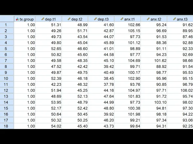
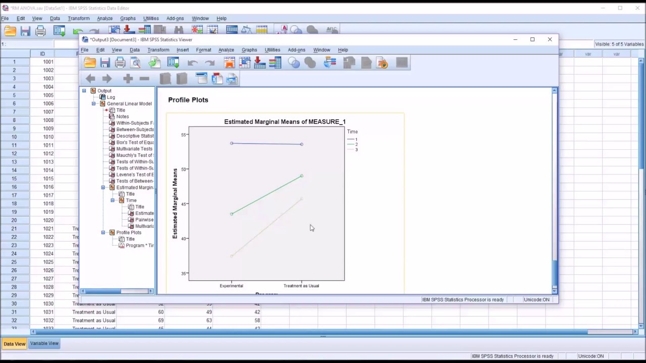
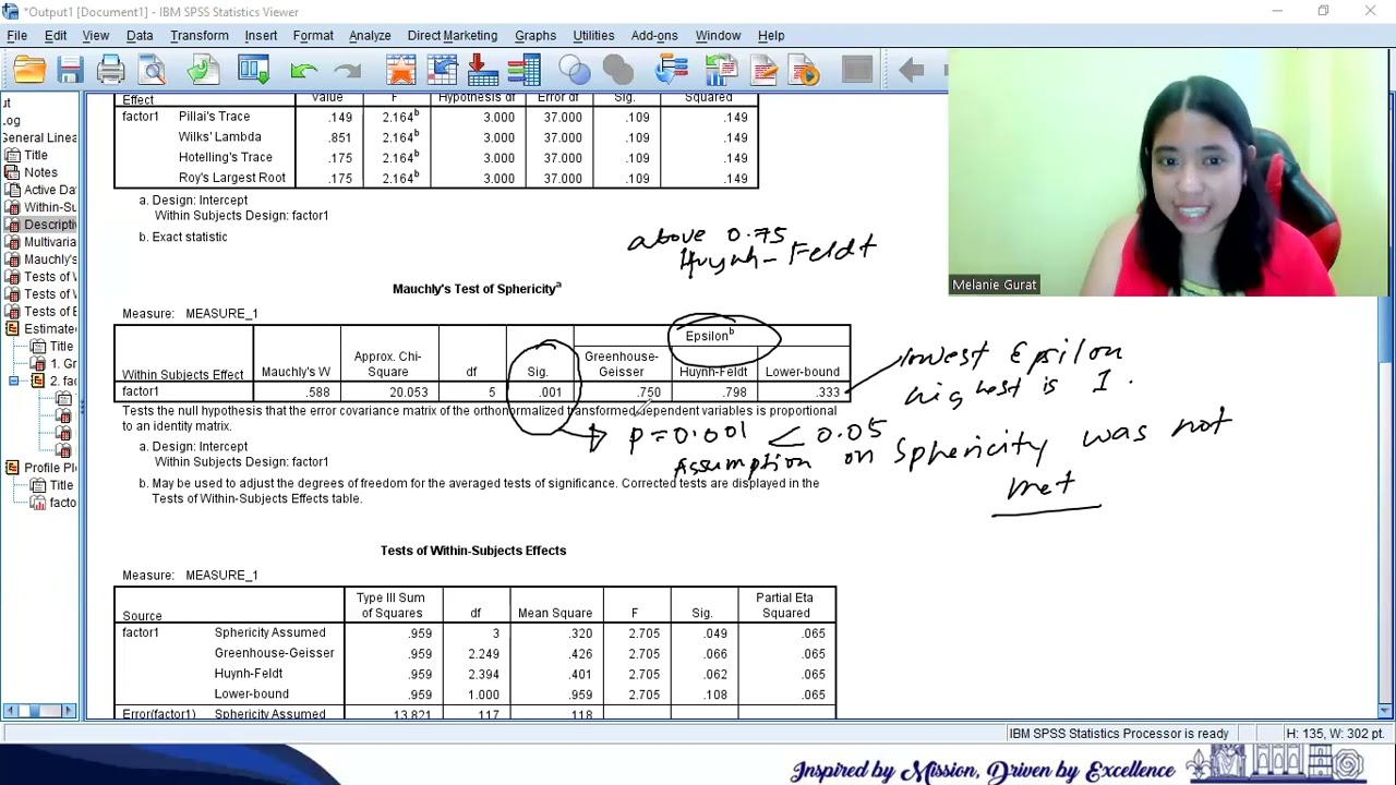
hi everyone in this video I'm going to demonstrate two-way repeated measures ANOVA when you have one between-subjects factor and one within-subjects factor and we will be focusing in on SPSS so also let me note that underneath the video description you will find a link to the SPSS data file used in this video presentation you'll also find a link to a supplemental PowerPoint that I will be referring to during this presentation so be sure to download both to follow along so let's get started so in a previous presentation I discussed and demonstrated the use of repeated measures analysis of variance when you measure an outcome variable repeatedly within a single group but it's oftentimes the case that repeated measures analysis is applied to data involving more than a single group so this approach for instance may be used in cases where the researcher hypothesizes that the variation in means associated with repeated measurements on the outcome varies across groups and this effectively translates into a hypothesis concerning an interaction effect between the repeated factor and a grouping variable so one might adopt this approach when testing whether differences in means observed over time are the same or different across levels of a grouping variable and if differences are found it's possible to examine whether the mean differences reflect different trends over time this can be particularly handy if one of the groups being compared as a control condition and other conditions are experimental in nature this approach could also easily be used when testing whether individuals react the same or differently across levels of a repeated factor and a grouping variable and basically with the repeated factor representing a reflecting different stimuli to which a person is exposed now for our current example the between-subjects factor is going to be treatment group which is coded one for control group two for treatment a and three for treatment B and we are going to test whether there are significant mean differences in anxiety scores over three measurement occasions as well as whether there are group differences in terms of how the means vary over time so here I've opened up my data and you see I've got the between factor which is treatment group just taking a quick look at it you can see one is control two is treatment a and three is treatment B and then we also have our repeated measurements with respect to anxiety so it's anxiety at time 1 time 2 and time 3 so let's go ahead and carry out the basic analysis by clicking on analyze then general linear model and repeated measurements or repeated measures under within subject Factor name I'm just going to go ahead and give it a name called time and number of levels is 3 because we have three measurement occasions so I'll click Add under measure name I can give it a give the repeated measures a name so I'll just call it anxiety and then click Add right there and then define so we'll move treatment group to the between-subjects factor box and then anxiety t1 t2 and t3 I'm going to move over to the within subjects variables under options I'm going to click on descriptives effect size power and also homogeneity test since now we have a between subjects factor then I'm going to click on estimated marginal means and I'm going to highlight all of these and move them over to the display means box and since I want to also incorporate pairwise comparisons of means between the different time points I'm going to click on compare main effects and then select bonferroni so next we'll click continue and then under post aux if you want to look at between group differences overall with respect to anxiety we can move treatment group over here to the Box on the right and then click on - key to get that under plots I'm going to select time and move it to the horizontal axis and click on add and then also I want to plot out any type of interaction that might occur between time and treatment group so I'm going to move time to the horizontal axis and treatment group to separate lines then click on add where it says chart type I'm going to leave it as bar as line chart if you want air bars you can also click on that so we'll click on continue and then on ok our output so you can see we have our descriptives we have multivariate test results that are given there's our univariate test results and so forth so rather than kind of going through all of these in the output file which is a little bit difficult to read I'm going to refer back to my powerpoint in describing the results so in terms of the first part of the output you can see that we have sample sizes as well as the means and standard deviations so with with the descriptive statistics you can see that we have the means in terms of anxiety at time one for the control group treatment a treatment B then at time two for the three groups and then at time three okay so the next part of the output contains multivariate test results so you'll see down here we've got multivariate tests and these are can be used to test the main effect of time and then also the time by treatment group interaction there's also another set of tests which contain univariate test results to do essentially the same thing now with respect to the multivariate tests it does make an assumption which is called the equality of variance covariance matrices and in the context of our our current model we're essentially looking at the variances and covariances of different scores between or across the groups so essentially if this test result right here is statistically significant and that can call into question the validity of our interpretations with respect to the multivariate test result but it is important to know that this test which is boxes tests is sensitive to multivariate and non normality and it can actually increase the rejection rate in terms of that particular assumption so basically concluding that the assumption is violated when perhaps it's not also the multivariate test results are fairly robust when you have equal or nearly equal ends in your groups so in other words if you have a ratio that's less than ratio of the largest end the smallest end this is less than 1. 5 then the the test tends to be more robust and that actually tends to be the in our current in our current situation so you can see right here I've outlined the test results with respect to time and time by treatment groups so there are four different multivariate tests results that are presented Wilks lambda tends to be one of the more commonly presented results so you can see right here that we have Wilks lambda for the main effect of time that effect is statistically significant and then the time by treatment group interaction effect is statistically significant so it's basically telling us that the variation in means on anxiety over the repeated measurement occasions is itself varying as a function of treatment group membership okay so in the next part of the output you can see that we have these tests of within subjects effects and so that's for the main effect of time and then also the time by treatment group interaction so as you can see we have two sets of tests that we could refer to theoretically we could refer to the multivariate test results or we could refer to these univariate test results the multivariate test results and the univariate test results both make assumptions concerning independence of observations and normality the multivariate test result makes no assumption concerning a condition referred to as ferocity whereas the univariate result does make that particular assumption and in the context of the univariate test violations for a state can translate and to increase type 1 error rate now there are a couple of ways in which we could assess us ferocity in this particular table above one is to utilize multis test so you can see right here we have a p-value that's given the sig right here and if this is greater than say point zero five the conventional threshold and that would be an indication that we have its ferocity being met the only thing about this test is that it is affected by non normality and it's also impacted by sample size so it does make this test a little bit untrustworthy at time so for that reason other authors have various authors have suggested just using the greenhouse geyser and in particular just using some rules of thumb for judging the level of departure from its ferocity so basically this epsilon parameter value of 0. 9 36 that is and essentially kind of an estimate regarding the degree of departure from its ferocity and an epsilon value that is equal to one would be consistent with ferocity so in a nutshell you'll notice that in these tests down here we have stress the assumed greenhouse geyser in wind felt both for the main effect of time and then also for the time by treatment group interaction so if you can assumes Frisky you know and this number right here is pretty darn close to 1 and you know obviously taken in conjunction with this result right here for Mosley's test I would indicate that we have as first e being met in that case we could focus our attention mainly on reporting on this forest e assumed output so you can see it's statistically significant with respect to time and then also for the time by treatment group interaction now if we have a more substantial departure from ferocity then as I noted before that could increase the type 1 error rate and so these other tests at Greenhouse geyser and wind felt for for that's shown in the Tesla within-subjects affects those incorporate adjustments to the degrees of freedom for those particular tests and basically makes these tests more conservative than this first the assumed test so if it's the case where we are concerned about a violation of ERISA T then we might want to go to either the green house geyser or the wind felt test now various authors have suggested you know some rules of thumb regarding which tests to use under which conditions so one rule of thumb is that if you have a green house geyser epsilon value that's shown up here this less than 0.
75 then you should go to the green house geyser spent with respect to that repeated-measures anova if you have a value that falls between 0. 75 and 1 then you would go to the wind felled option right here or if you don't feel like you have a really substantial departure from spur st then you could just stick with this for a c' assumed right here so you can see in this particular case our greenhouse Gaiser epsilon value is 0.