False Discovery Rates, FDR, clearly explained

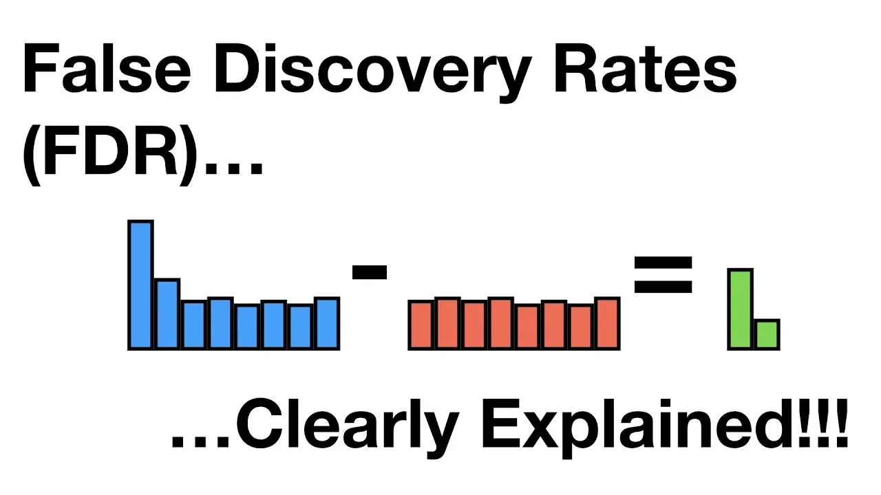
holy freaking smokes what it's time for stat Quest hello and welcome to stat Quest stat Quest is brought to you by the friendly folks in the genetics department at the University of North Carolina at Chapel Hill today we're going to be talking about false Discovery rates or FDR if you've ever seen or done anything with high throughput sequencing chances are you've heard false Discovery rates FDR before you may have even used them but where do false Discovery rates come from and how do they work before we get down to the nitty-gritty let me blurt out the main idea of this whole stat Quest false Discovery rates are a tool to weed out bad data that looks good now let's get down to the nitty-gritty let's start with an example of measuring gene expression using RNA sequencing here we're going to plot the measurements or the read counts for a gene called Gene X which is an imaginary gene on a graph with the y axis being Gene counts and the xaxis being the samples for this example imagine that we are looking at normal wild type mice later on we'll be comparing them to mice that have been treated with a drug isn't it funny that normal mice are called wild type if someone said I was a wild type I don't think they would also think I was normal anyway here's our measurement for the first mouse that we do this RNA sequencing on and here's the measurement for the second mouse that we do the RNA sequencing on RNA sequencing isn't perfect and different samples are always a little different so each time we measure expression we'll get slightly different values here's the measurement for the third Mouse and here are the measurements for a bunch of mice if we measured all normal mice we'd be able to calculate the average for all normal mice most of the values are going to be close to the mean rarely we'll get a value that is much larger than the mean and rarely we'll get a value that is much smaller than the mean we can summarize the distribution of the measurements using this bell-shaped curve most of the measurements which are close to the mean will come from the middle of this curve the rare measurement that is significantly larger than the average would come from the right side of the bell-shaped curve and the rare measurement that significantly less than the average would come from the left side of the bell-shaped curve now imagine that we do RNA seek on three mice collectively we'll call these three measurements sample number one because these measurements are close to the meain they come from the middle of the distribution now imagine we compare sample number one to another three measurements taken from normal wild type mice we'll call these new measurements sample number two again these three measurements come from the middle of the distribution if we did a statistical test to compare sample number one to sample number two the P value would be large greater than 0. 005 because the two samples overlap very rarely we'll get two samples that do not overlap when this happens the P value will be less than 05 this is called a false positive because the small P value suggests that the samples are from two types of mice or two separate distributions and this is false normally false positives are rare unless you're a packer but that's another stat Quest already on YouTube anyways normally false positives are rare 95% of the time the two samples will overlap this will result in a P value greater than 0. 05 5% of the time they don't this will result in a false positive with a P value less than 05 but human and mouse cells have at least 10,000 transcribed genes if we took two samples from the same type of mice and compared all 10,000 genes well 5% of 10,000 equals 5 00 false positives that means there will be 500 genes that appear to be interesting even when they are not 500 false positives is a lot can we do something about them the false Discovery rate can control the number of false positives technically the false Discovery rate is not a method to limit false positives but the term is used interchangeably with the method me in particular it is used for the benjamini hogberg method now there's a high probability that I just mispronounced benjamini or hurg and if I did I apologize before we talk about the details of the benjamini hosb method let's review the concepts that it's based on we'll start by generating 10,000 P values from samples taken from the same distribution that is to say we'll start with test number one and we'll use wild type mice and we'll take two samples from them we'll then compare the two samples with a statistical test and calculate the P value in this case the P value is large it's 0.

83 this is exactly what we expect because both samples are taken from the same type of mice and then we repeat the procedure for test number two and calculate another P value this time at 0. 98 again this is as expected to make a long story short we just repeat this procedure 10,000 times no big deal here I've drawn a histogram of the 10,000 P values generated by testing samples taken from the same Distribution on the X AIS we have possible value for p values on the Y AIS we have the number of P values in each bin 510 P values or 5. 1% are less than 005 close to 5% of the P values are between 0.

5 and 0. 1 actually each bin contains about 5% of the P values about 500 P values per B since the p values are uniformly distributed there's an equal probability that a test P value falls into any one of these bins now let's look at how P values are distributed when they come from two different distributions and by two different distributions I mean two different types of mice or we have wild type versus knockout or control versus drugged we're just comparing two different situations like before we start off with test number one but now we have two different distributions the black distribution is for our control mice the red distribution is for mice that have been treated with a drug in this example the drug increases this Gene's transcription like before we take two samples since the sample are now coming from two separate distributions there's a higher likelihood that the two samples will be separated and not overlap when we do the statistical test in this case we get a P value that equals 0. 03 and then we do the exact same thing for test number two notice that both of the P values are less than 05 so they're statistically significant since the samples were taken from two separate distributions this is what we'd expect like before we repeat this process 10,000 times here I've drawn a histogram of the 10,000 P values generated by testing samples taken from two different distributions most of the P values are less than 05 this is what we'd expect the P values greater than 0.

05 are false negatives from where the samples overlapped you can reduce the number of false negatives by increasing the sample size to summarize what we know so far when the samples come from the same distribution the P values are uniformly distributed but when the samples come from different distributions the P values are heavily skewed and closer to zero now imag imagine we're doing an experiment where we are testing all of the active genes in neuronal cells one set of neuronal cells is treated with a drug the other is not the drug might affect 1,000 genes the measurements for these genes will come from two different distributions the black sample is from the control cells and the red sample is from the cells treated with the drug since the samples come from different distributions the P values are skewed the remaining 9,000 active genes might not be affected by the drug this means the measurements for most of the genes will come from the same distribution the P values for these genes should be uniformly distributed the histogram of P values we obtain from all 10,000 genes is the sum of the two separate histograms the uniformly distributed P values come from the genes unaffected by the drug the P values on the left side are a mixture from genes affected by the drug and genes unaffected by the drug by I we can see where the P values are uniformly distributed and determine how many tests are in each bin here I've drawn a line indicating that about 450 P values are in each bin in the uniformly distributed part of the histogram we can extend this line and use it as a cut off to identify the true positives since we usually use a cut off of 05 we're going to focus on these P values roughly 450 P values less than 05 are above the dotted line and roughly 450 P values less than 05 are below the dotted line one way to isolate the true positives genes affected by the drug from the false positives would be to only consider the smallest 450 P values this procedure Works fairly well because the p values within the bins are skewed for the genes affected by the drug note this histogram is for p values between 0 and . 5 and spread evenly for the genes not affected by the drug bam if you can understand these Concepts then you understand more about false Discovery rates and the benjamini hochberg method than most people who use it all benjamini and hochberg did is convert this procedure that we just did by I into a mathematical formula so now let's talk about the details of the benjamini hochberg method like I just said it's based on the eyeball method we just saw the benjamini hurg method adjusts P values in a way that limits the number of false positives that are reported as significant adjust P values means that it makes them larger for example before the false Discovery rate correction your P value might be 0. 04 I.

E significant after the FDR correction your P value might be 0. 06 no longer significant if your cut off for significance is FDR values less than 0. 05 then less than 5% of the significant results will be false positives in other words these are the genes with P values less than 0.

05 the black box shows the genes with FDR modified P values less than 0. 05 notice that not all of the true positive genes are inside the Box however only 5% of the modified P values in the Box are false positives the remaining 95% are true positives why don't all of the true positive genes have adjusted fdrp values less than 0. 05 because not all true positive genes will have super small P values here's the histogram of true positive P values less than 0.

05 these genes on the right side of the histogram probably won't remain significant after adjustment surprisingly the math behind the benjamini hochberg method is simple let's take a look let's start with another simple example we'll take 10 pairs of samples taken from the same distribution I. E 10 genes that were not affected by the drug and here are the P values from those 10 tests the first thing we do is we order the P values from smallest to largest notice that one of the P values is a false positive that is to say it's less than 0. 05 let's see what the Benjamin hochberg method does to it the second step is to rank the P values and Let's Make spaces for the FDR adjusted P values that we're going to create the largest FDR adjusted P value and the largest P value are the same the next largest adjusted P value is the smaller of two options either the previous adjusted P value which in this case equals 0.

91 or the current P value times the total number of P values divided by the P Val rank in this case the current P value is 0. 81 the total number of P values is 10 and the P value rank is nine plugging these numbers in we get 0. 90 since we select the smaller option we're going to go with 0.

90 for the next largest adjusted P value we just repeat step four that is to say we select the smaller of these two options plugging in the numbers gives us the choice of 0. 90 or 0. 89 since we use the smaller value we go with 0.