[Music] hello everyone welcome to this lecture in the build large language models from scratch Series this is the second part of the multihead attention lectures in the previous part we looked at implementing multi-head attention in the following way what we did is that we had the input tokens so let me show you this figure which summarizes Everything yeah so this was the input Matrix which we had essentially the number of rows here represent the number of tokens which we have and each token was encoded as a three-dimensional input embedding Vector right in the first part
of the multi-ad attention what we essentially did was we created multiple weight matrices for the query key and the value so if we have two attention heads we'll create two weight matrices for the query Two weight matrices for the keys and two weight matrices for the values and then we will multiply the inputs with these weight matrices to get two queries two keys and two values so the main problem with this approach is that here you can see that there are two Matrix multiplications which are needed as we saw earlier gpt3 used 996 attention attention
heads so if you have 96 attention heads you'll need 96 multiplications to get the queries Matrix 96 multiplications to get the keys Matrix and 96 multiplications to get the values Matrix that's not very efficient right so today what we are going to see is that how can we make sure that the number of multiplications are reduced in particular what if we just need to do one multiplication for quick Keys one one multiplication for queries and one multiplication for values and then once we do one multiplication then we can split the Queries again into two parts
we can split the keys into two parts and we can split the values also into two parts for two heads and then we can perform the rest so once we get the copies or the multiple matrices for queries keys and values what we can do is multiply queries with keys transposed to get the attention scores then we can get the attention weights and we can multiply them with the values to get the context vectors so the rest of the procedure can Be bit similar but what if we can reduce the number of Matrix multiplications at
the start this is what we are going to look at in today's lecture so let's get started this procedure is called implementing multi-head attention with weight splits and it's definitely much more efficient than the multi-head attention which we saw previously so in the previous lecture the way we implemented multi-head attention was something like this we had the the Causal attention module and we calculated the causal attention module result which is the context Vector the context Vector for every single attention head and then we concatenated the results from the different uh context vectors together and that
led to a large Matrix this was the process now what we are going to do is we are going to follow a slightly different procedure and that's called multihead attention with weight splits and it's much more Computationally efficient so the main idea is that in the previous code we had maintained two separate classes we had maintained a class for the multi-head attention rapper and we had maintained a class for the causal attention and then we combine both of them into a single multi-head attention class so here in the in the top what you can see
over here is what we did previously We performed two Matrix multiplications to obtain the two query matrices q1 and Q2 Q2 what we are going to do right now is what if the weight Matrix which we start start out initially itself was a larger weight Matrix and then uh we multiply the inputs x with the query Matrix to get the queries and then after that we split the queries into two components so here you see the difference in the previous case we multiplied x with wq1 and we multiplied x with Wq2 but what if we
multiply x with a WQ which is already a large Matrix which consists of D out so here you see the dimensions of this initial weight Matrix are larger and that these Dimensions already include the number of heads so this Dimension 4 is the D out which is two multiplied by the number of heads so this D out is already specified before so the weight Matrix for the queries keys and the values which we specify already will kind of include the head Dimension and then we when we get the queries keys and values we'll split them
based on the number of heads so here we can see where we split the queries Matrix into two q1 and Q2 because there are two heads so ultimately the rest of the procedure will remain the same but we are just reducing the number of Matrix multiplications so if you look at this weight Matrix right now the number of attention head is specified Right uh so how is it specified so D out is equal to 4 and D out is equal to head Dimension multiplied by the number of heads so the head Dimension is equal to
2 because each head has a dimension of two this is what we had done here each head had a dimension of two each attention head here you see D out equal to two which was implemented in the previous case so each head had a dimension of Two And there are two heads so the D out in This larger trainable Q Matrix already includes number of heads I'll explain to you in detail what this means right now if you just get an intuitive idea of what we are trying to do that will be very helpful okay
so now uh let us get started with the code so we are going to implement multi-head attention with weight splits right so instead of maintaining two separate classes so here you can see earlier in our code we had the we had a Causal attention class which did all the computations of attention scores attention weights Etc and then we integrated this causal attention class with the multi-head attention rapper so we had a multi-head attention rapper and we created multiple instances or multiple causal attention objects within this rapper now the idea is instead of maintaining two separate
classes why don't we combine both of these Concepts Into a single multi-head attention class also in addition to just merging the multi-head attention rapper with the causal attention code let's make some other modifications to implement multi-head attention more effectively so as I told you earlier in the multi-ad attention rapper which we had earlier multiple heads are implemented by creating causal attention objects and uh the causal attention class independently performed the Attention mechanism earlier and then the results from each attention head were effectively concatenated now we are going to implement a class which is called as
multi-head attention class and we are going to integrate the multi-head functionality as well as the causal attention functionality everything within a single class the way we are going to do do this is that the this class splits the input into multiple heads by reshaping the Query key and value tensors let's see what this means don't worry about this sentence in this lecture I have constructed a Hands-On example so that you understand the code which we are about to write so first let's look at the multi-ad attention class and how we are going to Define it
this code right here which I'm showing on the screen is at the heart of the Transformer mechanism so you see we have the in init Constructor which is invoked by default And then there is the forward method at the end of the forward Method All We are going to do is calc calculate the context Vector for each of the input embedding vectors but what happens in the middle that is the main key which you really need to understand okay so I could have just taken you through this code but I have seen that if I
take students through this code it becomes very difficult for them to wrap their heads around what exactly is going on Especially because if you see the dimensions there are four dimensional tensors which are involved in this code and there is a very good reason for why we need four dimensional tensors so if you if you just go through the code you will you will think that you have understood it but you would not have because there are lot of subtleties with respect to the dimensions so what we are going to do is that we are
going to go to the Whiteboard and I constructed this Example completely from scratch so we are going to take a simple example we are directly going to start from the input and we are going to do all the steps on the Whiteboard which are implemented in this code then you will find that understanding the code is extremely easy at every step of the code I'm going to take you to the Whiteboard and I'm going to explain to you what exactly is going on okay so let's get started I've tried to distill this down To 11
steps and uh I I will explain everything related to matrices Dimensions extremely clearly I will not assume anything everything is written down on the Whiteboard so that you will not be afraid of this code I have seen several other YouTube videos and even lectures where uh people just explain this as if it's very easy to understand but you need to decompose it into individual layers and explain every single one of them okay so I'm going to Start with the forward method and I will explain every single line here step by step so first the forward
method takes the input X right let's see what that input looks like and what it means so the first step to the attention make the multi-ad attention with weight splits that code or the multihead attention class is that we have to start with the input the way we will specify the input is that the input has three dimensions the First Dimension is the batch the Second is the number of tokens and the third is the input Dimension right what is this D in the D in is basically every token is represented by a vector embedding
so this D in is the dimension of that Vector embedding so 1A 3 comma 6 means that I have three tokens you can think of one token as one word for Simplicity so let's say the three tokens are the cat Sleeps let's say these are my let's say these are my three words then what we are essentially doing here is that we are converting each of these words we are converting each of these words into six dimensional vectors so the will be a six dimensional Vector which is the first row so which is the first
row over here so look at the first row over here this is the six dimensional Vector for the this is the six dimensional Vector for cat and this is the six dimensional Vector for sleep so you'll see that this is a 1x 3x 6 for Simplicity I have taken the batch size equal to 1 okay so this is a 1x 3x 6 tensor why 3x 6 because we have three rows here and we have six columns uh each row consists of six six dimensional vectors so I hope you have understood how the input has been
defined so here you can see the input shape is B comma number of tokens comma input Dimensions so I hope you you have Understood this okay now let's come to the next step the next step is what we have to do is we have to essentially decide two things we have to decide what our output Dimension is going to be and we have to determine the number of Heads This output Dimension is basically we have the input input embedding Vector for each token right ultimately we will get a context Vector for every token so ultimately
similar to this input embedding Matrix which is 3x which is 3x 6 we will have a context embedding Vector which is three because we have three tokens multiplied by D out so now we have to also decide what is D out which is the so each each token will have a context vector what is the dimension of that Vector we have to decide so now I am deciding that D out will be equal to 6 which is same as D in this is typically done in GPT based models the D in and the D out
are the same second thing we also have to decide Is how many attention heads do we want to have so I have decided that we are having two attention heads right now in GPT the number of attention heads are 96 and the D out is also pretty large but exactly what we are doing right now can be scaled to a larger D out and larger number of heads okay so I'm using D out is equal to 6 and number of heads equal to three so then each head will have a dimension which is called as
head dim and we'll look at that also later each Each head will have a dimension of head dim which is equal to head dim which is equal to essentially the D out divided by the number of heads which is equal to 6 / 2 and that will be equal to three so then the dimension of each head is equal to three and since there are two heads the total D out will be equal to six okay so this is the second decision point the third decision point which I have to make is that I have
to Initialize or it's not a decision Point rather but it's the third step so the third step which we have to do is initialize trainable weight matrices for the key query and the value so we have to initi w k WQ and WV okay so remember that the input which we have which for now can be thought to be six rows and three columns has to be multiplied sorry three rows and six columns so the input is three rows and six columns so when you Construct these trainable weight matrices for the keys query and value
their first Dimension has to be equal to D in because if you look at the input Dimension the input the number of the last dimension of of the input is D in and for these for d for this input to be compatible with this WK WQ and WV in multiplication you need the first argument here to be equal to D in so actually the dimensions of the trainable key query and value matrices Are D in multiplied by D out which is 6 by 6 because D in is equal to 6 and D out is equal
to 6 so we have to initialize the these three vectors these three matrices rather and I have shown these random initializations here so you can see that WQ is a six diens or a 6x6 tensor WK is a 6x6 tensor and WV is a 6x6 tensor let us let me show you in code where these matrices are actually initialized so if you look at the code these matrices are actually initialized In the init Constructor so w query W Key and W value these are trainable weight matrices as you can see the dimensions are D in
D out and we are using the linear layer of neural networks with the bias equal to zero to set the uh initial values for these why do we use a neural network linear layer because it's optimized for initializing the weights so it's much better when we do the back propagation later so this is where the the trainable weight matrices for query Key and value are initialized in the init Constructor so it's called by default when we create or it's these Matrix are created by default when we create an instance of the multihead attention class all
right so up till now we have essentially initialize these trainable weight matrices w k WQ and WV Now we move to step number four step number four is the step from which computations actually start so we have the input now Right and uh we have the these matrices we have trainable Keys the trainable queries and the trainable values what we'll now be doing doing is that we will multiply the input with these matrices to ultimately get the keys the queries and the values so what are the dimensions of the input the dimensions of the input
are one one M uh me just write this again the dimensions of the input are 1 multiplied By 3 because we have three rows multiplied by six columns correct and the dimensions of each of these qu key query and value trainable weight matrices are six which is D in multiplied by 6 which is D out so when you multiply the input with these weight matrices the result which you'll get is 1x 3x 6 so you'll get the keys you'll get the keys Matrix which is 1x 3x 6 you'll get the queries Matrix which is 1x
3x 6 and you will also get The values Matrix here which is 1x 3x six let's try to understand what this 1 3 and six is so I as I've written over here one is the batch size which we are taken to be one three is the number of tokens because we have three tokens and D out is basically the output Dimension so the way to interpret these keys saries and value Matrix is that each row basically corresponds to one token so the first row corresponds to the first token the second row corresponds to the
Second token and the third row corresponds to the third token and there are six dimensions in each row because each token is a six dimensional representation because D out is equal to 6 now let me show you in the code where this is calculated so if you go down below here you see the keys queries and values what we have done is that we have passed in the input to this neural network linear layer so what this does is that the Trainable weight mates for the key query and value are applied on this input and
we get the keys queries and the value Matrix as we saw on the Whiteboard the shape of this is B which is the batch size the number of rows is equal to the number of tokens and the number of columns is equal to the D out which is equal to six okay now we move to the next step and this is the step where four dimensional tensor start to come into The picture right so until now we have three dimensional tensors for the keys queries and values right why the fourth dimension needs to come into
the picture is that until now these three dimensions are for batch size number of tokens and D out but there is no dimension for the number of heads uh or the head Dimension rather so this is where we come to next so what we are now going to do is that we are going to unroll the last dimension of the keys Queries and values to include the number of heads and the head Dimension what this means is that if you look at this last dimension of the keys here in fact even for queries and values
this is D out right and D out is essentially number of heads into head Dimension as we have seen earlier so let me take you yeah so here remember what we saw head Dimension is equal to D out divided by number of heads so D out is equal to head Dimension multiplied by the number Of heads so that's what we are actually going to do we are going to unroll the last dimension of the keys saries and values to include number of heads and head Dimension right so we have D out which is equal to
6 which is a decision which we have made and we have also made a decision with respect to the number of attention heads which is equal to two So based on these two decision points the head Dimension is Fixed and the head Dimension will be equal to 6 / 2 which is equal to 3 so what we are going to do next is that we had this 1X 3x 6 matrices right for the key SAR and value now we are going to roll them into 1 by 3 by 2 by 3 so now instead of
D out we will have number of heads which is equal to two and head Dimension which is equal to three so let's see what the reshaped keys queries and values Matrix actually look like uh so when you reshape the Keys queries and value Matrix they start looking like this and I'll tell you how to interpret four dimensional tensors also so for the sake of Simplicity uh let's first analyze the queries Matrix so this Matrix is 1x 3x 2x 3 how do you Analyze This four dimensional tensor for now forget about the first which is the
number of batches okay so next look at three so this three is the number of rows so this is my first row and uh this is my first token also Right this is my second token and this is my third token correct that's why there there is this three now let's look at this two what is this two this two is the number of heads so if I go in each token right now let's see if I go in first if I go in the first token the first row corresponds to the first head and
the second row corresponds to the second head that's why there is this two and if I go within each head I'll see that There is there are three dimension the First Dimension the second dimension and the third dimension so remember the head Dimension is equal to three so the way to interpret this Matrix is start from the outermost value so three why three because there are three tokens then go to each token why two because there are two heads in each token then go within each head why three because the dimension of each head is
three each head is a three dimensional Vector so in this same way we can analyze the queries the keys and the value Matrix also so the keys Matrix will also be uh 1X 3x 2x3 and the values Matrix will also be 1X 3x 2x 3 as I mentioned before let me repeat it again each row over here is a token so if you look at the value Matrix let's look at the second row the second row corresponds to the second token if you now look at the first row of the second row this that is
the threedimensional Head Vector for the first head if you look at the second row that's the three-dimensional head Vector for the second head remember every token has two attention heads so you can think of as two people paying attention to each token token because we have two attention heads that's why there are two rows corresponding to every token now if we come to the code this line has been mentioned over here so see we have to unroll the last Dimension so Now the D out will be replaced with the number of heads and head Dimension
so this is exactly what has been done over here keys. view so now keys will be replaced with keys do view B common number of tokens common number of heads and head Dimension this is exactly uh what we we just saw on the Whiteboard so in this step the three dimensional tensors have been converted into four dimensional tensors to include the number of heads and the head Dimension Great now we move to the next step so if you see uh if you see this let's look at this argument which is three um so the shape
of this is 1A 3A 2 comma 3 right now let's look at this first this this entry this is three now this three is the number of tokens which means that currently these matrices are grouped according to number of tokens right so I'm saying that this is the first token this is the second token and this is the third Token and then I further dive into number of heads and the dimensions in each head but it turns out that later when we want to compute the attention scores the only way the computation can proceed ahead
is if we Group by the number of heads so instead of grouping by the number number of tokens I actually want to group by the number of heads and we have two heads here right so I want to flip these Dimensions I want to flip these Dimensions here so that the first row represents the first head the second will represent the second head and each will have a 3X3 let me show you what I mean so now what we are going to do is we are going to group The matrices by the number of heads
okay so currently the keys queries and the values Matrix have the dimensions of one which is the batch three which is the number of tokens two which is the number of heads and three which is the head Dimension so We are grouping with respect to the number of tokens but now I want to group with respect to number of heads so again I want to switch the dimensions to be I want to switch this this to uh let me write it again yeah I want to switch this two with three and this three should come
over here so I want the the matri to have the dimensions of B comma number of heads comma number of tokens and head Dimension so I want the dimensions to be 1 comma 2 comma 3 comma 3 so what I'm going to do in the code also you'll see we are going to transpose keys quaries and value and we are going to transpose one comma 2 now why do we do one comma 2 over here because python has zero indexing so index zero is this since we want to Interchange the number of tokens and the
number of heads the indexes which we need to transpose are index number one and index number two that's why we are doing Keys queries and value And transpose 1A 2 so let's see what the result actually looks like so when you when you make the 1A 3A 2A 3 to 1A 2 comma 3A 3 now the transposed queries keys and Valu start looking like this and now you will see that they are grouped by head so the first thing what we can do is that let's look at this block in the queries so we are
analyzing the queries Matrix now the shape of the queries Matrix is what 1 Comma let me write it here again 1 comma 2 comma 3 comma 3 right that is the essentially the shape of the queries Matrix and we are going to analyze this so let's start with this two which is the number of heads so if you look at the first block here uh let me erase this right now now and then draw it again yeah so if you look at the first block over here which are marking with these curly braces That's the
first head if you look at the second block here that's the second head so see now this two because this two comes over here now we can group with respect to number of heads so the first block shows everything with respect to head one and the first row over here is the first token the second row over here is the second token and the third row over here is the third token similarly if you look at head number two the first row is the first token the second row is The second token and the third
row is the third token so now we have the dimensions as number of tokens and head Dimensions come last so each token if you see each token has a three dimensional Vector because the head Dimension is equal to three so the the reason this helps is because since we can now group with respect to heads we can compute the attention score for each head separately so remember there is one attention score There are there is an attention score Matrix for the head one and there is an attention score Matrix for the head two and then
we we are going to U concatenate them together right so it makes sense to group with respect to the head and that's why this step exist this keys. transpose it's very difficult for students to understand this unless you see this visual example of why we are essentially doing this transpose the main reason we do do this transpose is That here you see we are grouping with respect to uh we are grouping with respect to number of tokens here but that's not good if you want to compute the attention scores for each head parall so we
group with respect to number of heads so that's why it's important to flip number of tokens and number of head Dimension and that's exactly what we have done okay now let's go to the next step the next step is to find the attention scores so remember Now we have the uh we have the queries Matrix we have the keys Matrix and we have the values Matrix in exactly the shape which we want so now we can do uh we can go ahead and find the key queries and the keys transpose to get the attention score
so let me show you how this is done first let me rub all of this okay okay so now I have rubbed all of this so what we are now essentially going to do is that um this is the Head number one right this is the head number one of the queries and this is the head number one of the keys so what this this shape will help us do is that when we do queries multiplied by Keys transpose it will directly uh take the equivalent product of head one of the queries with head one
of the keys and then head two of the queries and head two of the keys but remember when we take the keys transpose what's really important to us Is that now the shape of the keys is B B common number of head is common number of tokens and head Dimension so what it's really important to us is number of tokens and head Dimension so remember the formula for calculating the attention score is queries multiplied by Keys transpose right so here also we are going to do queries with respect to Keys transpose but what exactly do
we have to transpose we have to Transpose uh we have to transpose this so we have to transpose the last two dimensions and let me show you what that transposed key Matrix looks like yeah so this is the transposed key Matrix now here you can see the key Matrix uh if you see the first row it's 4143 -1. 423 and - 2.71 31 right so when we do Keys transpose Keys transpose 2 comma 3 it will transpose along the last two Dimensions so now that that row which we Saw has now become a column over
here so this is the keys transposed and here is the queries Matrix and I've shown the keys transpose over here so the queries matrix dimensions is 1A 2A 3 comma 3 the keys transpose Dimension is 1A 2 comma 3 comma 3 so they they they are compatible for multiplication and the way the multiplication will now proceed is that the head one will only be multiplied by the head one of the keys transposed the head two here will Only be multiplied with the head two of the keys transposed and ultimately when we do this multiplication we
we will get the attention scores Matrix so this is the attention score Matrix which we have and the dimensions of this are B number of heads number of tokens and number of tokens let me show you why um okay so if you look at what we are multiplying here the query's dimensions are B comma number of heads comma number of tokens comma head Dimension right and When we do Keys transpose uh 2 comma 3 the dimensions here are B number of heads head Dimensions comma number of tokens so essentially you can think about it like
we are multiplying two matrices with the dimensions number of tokens comma head Dimension multiplied by head Dimension number of tokens so what will the resulted Matrix will have number of tokens rows and number of tokens columns and the first two Dimensions here will Stay the same because they are the same in both of these matrices we are multiplying so the resultant attention scores will have the dimensions of B number of heads number of tokens and number of tokens it's fine if you forget these Dimensions but you should be able to interpret what is going on
here so let's see what is going on here remember we have we are grouping with respect to head so that stays the same this first uh this first block which I've Highlighted right now that is head number one and the second block which which I've highlighted right now that is essentially head number two this is the first thing to understand okay then what we are doing when you look at the let's look at head number one for now if you look at the first row the first row essentially consists of the attention score between of
the first word with all the other words right so remember our sentence was The actually let me write it over here that will be much better so our sentence was the the cat the cat and here it was sleeps right the cat let me just write it over here yeah the cat sleeps and the same words I'm also going to write over here so the first row is let me write it over here actually The first row is the the second row is cat and the third row is sleeps so that's why the final two
dimensions are number of tokens comma number of tokens because if you look at the second row now if you look at the second row now the first element of the second row tells us information about the attention between cat and the the second element of the the second row tells us the information between cat And cat so if the query is cat how much attention should you pay to cat the third element here tells us the information between cat and sleep which means if the qu if the query is cat how much attention should you
pay to sleep so that's why the shape of the attention Matrix for every head is number of token rows and the number of token columns because an attention score exists between each token for every other token so whenever you see these Dimensions Right don't get confused by it try to always understand the meaning behind it that's why we had so many lectures on the attention mechanism before just so that when we reach this stage understanding all of this becomes easy so remember until this stage we have computed the attention score so this is exactly what
is done here remember what we saw on the Whiteboard to compute the attention scores we'll take the queries and we'll multiply with the keys. Transpose 2 comma 3 because uh in transposing 2 comma 3 we'll make sure that the correct queries and the attent and the KE transpose product is taken to calculate the attention scores and uh this is also implemented in the code so if you see in the code the attention score is the product is the scaled product between queries and the keys great so here it shown dot product for each head now
you'll understand why I'm saying each head because as I showed you before each head has number of tokens comma number of tokens attention scores and for for one head it's here and for the second head it's below okay now we come to the next step the next step is to essentially find the attention attention weights okay so uh if you look at this attention score over here right now you'll see that for every token there is an attention score with respect to every other token right but That's not what's the mechanism in causal attention what
causal attention says is that when you look at the you should only look at the attention score between the and what comes before it so the and the all the other elements here so let me show them with a different let me first rub this uh so that yeah so what causal attention mechanism dictates is that when you look at the first word which is the only the attention score between the and what Comes before it should survive so all of this should go to zero if you look at cat only the attention score of
the Words which come before so the and Cat should survive this should go to zero and when you look at sleeps attention scores of all Will Survive because all the words come before it this is what we are actually going to implement next so to do that first what we are going to do is we are going to take the attention scores which we have and Replace all of the elements above the diagonal with negative Infinity the reason we uh replace this with negative Infinity is because after this point we are going to implement the
soft Max function so that each row sums up to one and when we Implement soft Max whatever is there in the infinity will automatically go to zero so it will kill it will kill two birds in the same Stone we will implement the causal attention mechanism and we'll also make sure that All the rows sum up to one but before we Implement soft Max we do one more thing we divide every single element here with the square root of the head Dimension and this when we looked at the lecture for uh self attention we saw
why this is done this is essenti to make sure that the variance between the when we take the dot product between the queries and the keys the variance scales up with the number of dimensions and to prevent the variance from blowing up we have to Divide by the square root of the head Dimension this also makes sure that the values in the values before we compute the soft Max are not very high and that's generally useful for back propagation and leads to stable gradients so what we'll be doing is that the head Dimension as we
saw is three right because the D out is equal to 6 and the number of heads is equal to 2 so each head Dimension is equal to three so We'll divide this after replacing the elements above the diagonal with negative Infinity we'll divide this with square root of 3 which is square root of head Dimension and that leads to this Matrix over here or this tensor I should say and then we apply soft Max to this tensor so we make sure that every row here sums up to essentially so if you look at each row
in this you'll see that it it's summing up to one and the reason it sums up to one is we are applying Soft Max so now I can make claims interpretable claims so when I say that when I look at the second token cat I should pay 96% attention to the and I should pay 4% attention to cat when I look at sleeps I should pay 4% attention to the I should pay 26% attention to cat and I should pay pay 69% attention to sleeps remember these values are not optimized but when they are optimized
uh when we look at back propagation later uh the fact that these values sum Up to one will carry meaning because we can make interpretable statements such as what I was making right now remember that after we are going to apply soft Max uh the attention weights have exactly the same dimensions as the attention scores which is going to be the batch size number of heads number of token tokens and number of tokens so this is the dimension of the attention weights which is 1A 2A 3A 3 uh so if you look closely to go
from Attention scores to attention weights we actually M we actually have very we have a rich number of steps and it's important for you to understand all of these first what we did is we applied a mask so that all elements above the diagonal are negative Infinity then we divided by the square root of the the head Dimension then we applied soft Max this is how we got the attention weights now let's see how that is done in the code H before that one thing usually we Can also Implement Dropout after this so you can
mention a dropout rate which is actually one of the arguments in the multi-ad attention class but here I'm not implementing Dropout for the sake of simplicity so if you look at the code here we have got the attention scores the first step as I said is to create this mask and and then apply this mask to the attention score so that all the elements above the diagonal are negative Infinity that's what this step is doing Uh here the mask actually has also been defined over here see this is the upper triangular mask which is all
the elements about the diagonal one then they are replaced with negative infinity and that's applied to the attention scores so this will ensure that all the elements above the diagonal of the attention scores are equal to negative infinity and we are only considering context length here why context length because let's say context length is Three it means that maximum if three words are given we can make prediction of the next word so when we implement this Dropout mask we only Implement a mask of context length comma context length there is no point in implementing a
bigger mask because anyway we are not going to look at more tokens than the context length at a time and if it happens that we are looking at a batch where the number of tokens are less than the context size this statement makes Sure that then the mask stops at number of tokens but this is a detail which probably uh you can Overlook right now if you're understanding all the other things that's what the most important if you understand this Minor Detail it's awesome then the next step is to apply soft Max but as I
told you before applying soft Max we defi we divide every element with the square root of the head Dimension if you look at the keys. shape let's look at keys. shape uh This is going to be the keys do shape so keys do shape of minus one which means that we are going to look at the last Dimension which is the head Dimension so we are essentially dividing by square root of head Dimension here and then we apply the soft Max y Dimension equal to minus one because we need to make sure that all The
Columns of a row sum up to one and then as I said we can even Implement Dropout if needed towards the end so up till now we have reached a Stage where we have obtained the attention weights is basically and I hope you understand the meaning behind this final attention weight matrix it's not just important to understand how the dimensions work so to make sure you understand the meaning let me go through the meaning of this attention weight Matrix once more um this what I'm highlighting right now is the attention weights for the first head
this second block is the attention weights for the Second head in each attention uh head block you will see that the size is number of tokens rows and the number of tokens columns so each value is essentially the attention weight between let's say this is the attention weight between this is the attention weight between the second row which is the second token and the second token this is the attention weight between uh the third token as the query And the first token as the key so basically you'll see that every single element here has some
meaning it essentially encodes the attention weight between the query and the particular key okay now let's go ahead the last step which we are going to implement is that we have to calculate the context Vector remember the aim of all the attention mechanisms is to ultimately compute the context Vector Matrix and this is exactly what we are going to do and to Compute the context Vector Matrix we take the attention weights and we multiply them with values remember the value Matrix was The Matrix which we had computed earlier let me show you where the value
Matrix was in case you have forgotten it because we have done so many things uh yeah so here was the value Matrix which we had computed we have not used it until now it will only be used in this last Step okay so the attention weights will be multiplied by the values Matrix to get the context Vector Matrix so let's see how the dimensions work out here okay the attention weights as we looked earlier over here the attention weights have the dimensions of B comma number of heads comma number of tokens comma number of tokens
and as we saw earlier the values Matrix has the dimensions B comma number of Heads uh comma number of tokens and head Dimension so effectively let's see whether these matrices can be multiplied so this is number of tokens and number of tokens and that will be multiplied by number of tokens and head dim so the number of columns here is number of tokens and the number of rows here is number of tokens so the number of columns in the first Matrix are matching the number of rows in the values Matrix so we can see that
these two matrices Can essentially be multiplied so multiplication is possible and now let us see how the multiplication will actually work in practice this is the final attention weights Matrix here it's mentioned attention scores but I should have called it attention weights remember there is a difference between scores and weights attention weights in in the attention weights each row sums up to one that's not the case with attention scores okay so this is the Attention weights and this is my values this my values Matrix so this 1A 2A 3A 3 and this 1A 2A 3A
3 and when we multiply the resultant output will be B comma number of heads comma number of tokens uh comma the head Dimension so here you can see that the context Vector output is B comma number of heads comma number of tokens comma head Dimension which is 1 comma 2 comma 3 comma 3 Let's interpret this again uh so here you can see that there are two Heads so this is head number one and this is head number two and in each head there are number of tokens so if you look at each head there
are three rows so each row corresponds to one token but now if you look at what what each row represents each row represents the context Vector for that particular token and it has the dimensions equal to head dim because head dim is equal to three so that's the meaning of this uh context Vector Matrix which we have reached but Now remember there is a problem here right or not a problem uh but we have to somehow merge this number of heads and head Dimension back together because the resultant context Vector Matrix remember what we saw
earlier the let me scroll up a bit so if you if you if you looked at the goal which we had when we started this lecture the goal was that the resultant context Vector Matrix should have the dimensions of uh yeah as I mentioned to you the Goal was that the resultant context meor Matrix should have D out right as the dimension so we should again pull back the head Dimension and the number of heads together so that we can get the resultant Matrix which has the D out Dimension preserved uh whereas let's see what
we have obtained until now well until now the context Vector Matrix which you have obtained yeah the context Vector Matrix Which we have obtained has number of heads and head dimensions in separate positions so first what we'll do is that we'll bring them closer together so that we can then merge them to get the D out so what we are going to do is now we are going to swap this this number of tokens index with the number of heads index so that the dimension of the context Vector Matrix is so that the shape of
the context Vector Matrix is changed so the next step is basically Step number 10 and that is to reformat the context vectors So currently the context Vector shape is B comma number of heads comma number of tokens comma head Dimension right and I want the number of heads to come here so that they're closer to the Head dim and I want the number of Tok number of tokens to go here so I want the resultant Matrix to be B comma number of tokens comma number of heads comma head Dimension so essentially what I will do
Is after I compute the context Vector Matrix I'll do a transpose of the first index and the second index and so the resulting context Vector Matrix now which has the dimensions of B comma number of tokens comma number of heads comma head Dimension looks like this so here you see now the interpretation is different now this is my first token now the grouping is with respect to tokens this is my second token and this is my third Token and in each token there are two heads so if you look at the first token there are
two heads and if you look at the first head this is the vector with respect to the first head the context Vector context vector and the second row is the context Vector with respect to the second head for the first token now let's see how all of this is implemented in code actually all of what we saw right now is just implemented in one line of code but to understand this We really have to understand first of all how the attention weights are multiplied with values the multiplication really makes sense and why do we do
this transpose 1A 2 the reason we do this transpose 1 comma 2 is to get the context Vector mat in this shape the reason we get it in this shape is now you can see the number of heads and head Dimension are closer together so we can merge them um into the D out more easily so here you can see this is What we have reached until now where the context Vector is obtained and it's in the correct format now the last step what we have to do is that we have to um let me
show you the last step what we have to do is essentially we have to combine the results from multiple heads so see this is the context Vector Matrix which we have obtained right now right so if you look at the first token which I've highlighted over here this is the first Head and this is the second head now what I will do is that when I look at the first token I will combine these two together into one row so that it will be uh six the dimension will be six so so here these are
three and these are three right so I'll combine the outputs from both of these heads into one output so let's see how this looks like so then the first row will so then we'll flatten this is called flattening will flatten each Token output into each row so the head one and head two outputs are combined together so if you look at the final output the first row consists of merging of the two heads for the first token the second row consist of the merging of the two heads for the second token so for the second
row we merge these two out outputs into one single row and for the third token we merge these two outputs into a single row so you'll see that the F the this is the third row so this now What I what I'm showing on the screen here is my final context Vector Matrix and how to interpret this if you look at the first row the first row is the context Vector context Vector for the first token first row is the context Vector for the first token why does it have six elements because d out is
equal to 6 the second row is the context Vector for the second token and the third row is the context Vector for the third token so overall You see we first split the D out into number of heads and head Dimension and now we brought it back together to get the D out so in the final shape you will not see the number of heads it's all merged into this D out so this is my final answer right now and the shape of this is 1A 3 comma 6 which is B comma number of tokens
comma D out so this is exactly what is done here what we do is that we uh we take this context vector and we reshape it into B Comma tokens comma D out why this continuous is needed is because we want to make sure that when we reshape matrices they are in the same blocks of memory so when we reshape uh tensors let's say and if they're in different memory blocks it becomes difficult so first we make sure that using this continuous they in the same memory block then we reshape them so that the final
output is B which is the batch size number of tokens which is equal to three In the example we saw and D out which is the output Dimension which is equal to six and then there is an optional projection layer towards the end so if you look at the out out output projection it's again a linear layer and whose parameters can be learned this is not really necessary but sometimes it is implemented in practice now this is exactly the entire procedure for how the multi-ad attention is implemented from scratch and here we saw the multi-head
Attention for the example which we have so the first token is again the the the second token is cat and the third token is sleeps me write this again yeah the third token is sleeps so you see through this entire procedure we obtained the enriched context Vector representation for these tokens similarly when you deal with large volumes of text you take sentences you break them down into tokens then into Token IDs then into input embeddings and similar to this procedure you get context vectors for each token which you have ideally when we run the actual
code we will have multiple batches but I showed only one batch right now for Simplicity so uh to whoever who have reached until this stage I want to say that thank you for following with me for so to many lectures I know these lectures are becoming very long but unless I explain every single thing in Detail it's very difficult for you to understand all the details so congratulations if you have reached this lecture you have successfully understood how the multi-head attention works and I think there are very few people who really understand this entire piece
of code block by block okay so I'll share this notebook with you and whatever I explain to you on the Whiteboard all the steps which which I laid out in front of you on the Whiteboard uh all of those have been explained here as step one to Step 11 and uh I have explained added a detailed explanation of the multi-head attention class in today's lecture I did not just want to read this but I wanted to construct a practical example to show you how the dimensions actually work and uh it took me a long time
to make this example but now I think it's worth it because it really helped me explain it and I hope you understood it better so Now we can actually test out the multi-head attention class so here are my inputs uh as I showed you on the Whiteboard we have three tokens and we have six the embedding Dimension is six the only change here what I'm going to do I'm going to create a batch so I'm going to going to create a batch of two such inputs and I'm going to stack this batch on top of
each other so I'm going to assume a d out equal to six exactly what we saw on the Whiteboard and Context length equal to six and then we are going to implement the multihead attention class so D in is equal to 6 uh D out is equal so D in is equal to six right because each um each token has the input embedding dimension of six D out equal to 6 the context length which we are using is equal to uh six then uh yeah the dropout rate which we are considering is zero we can
even include the dropout rate so the dropout rate Will change this this last layer of Dropout and randomly block out some attention weights this is good for generalization and the number of heads equal to two so we create an instance of this class and then create the context Vector Matrix and you'll see for the first batch the context Vector Matrix has three rows and six columns let's see if the shape matches what we had seen on the Whiteboard Uh okay so let me scroll down below yeah this is the final context Vector Matrix which we
had obtained yeah so this also had three rows okay I think I need to scroll up a bit yeah this is the final context Vector Matrix which we obtained and this also had three rows and six columns the values might be different because we have done the initializations differently here I have taken random initializations in the python code there Are some other initializations every time you initialize we take from a goian distribution so the values might be different but let's check the shape so this is 3 comma 6 three rows and six columns and here
also we can see that three rows and six columns awesome so the shape matches but you'll see that since there are two batches here's the context Vector Matrix for the first batch and here's the context Vector Matrix for the second batch so the Multi-head attention class which we defined is extremely powerful because it can also handle multiple batches at once we can even do 50 data batches and then it will just have one 1 two it will have 50 such context Vector matrices okay that's it that brings me to the end of this section or
the end of this lecture so in this lecture we implemented the multi-head attention class that we'll be using in the upcoming lectures to implement and train The llm this code is fully functional but we we used relatively small embedding sizes and number of attention heads to keep the outputs readable so as I showed you we only use two attention heads but gpt3 actually was 96 attention heads so the smallest gpt2 model had 12 attention heads and a context Vector embedding size of 768 the largest gpt2 model had 25 attention heads and a context Vector embedding
size of 1600 and gpt3 has even higher so the gpt3 largest model has 96 attention heads I think and generally in GPT models the D in is equal to D out in the example which we saw D in was equal to D out equal to 6 but here the D in and D out are much larger around 768 Etc again thank you so much everyone for reaching the end of this attention series it's been one of the longest and most comprehensive series which I have covered and uh I really enjoyed learning About all of these
things I can see that many llm practitioners cannot understand these Dimensions or they do not take time to go through understanding the theory the building blocks behind how the attention mechanism Works they just implement the code bases which are available which completely abstract away all of these things so I don't think that's the good way or the correct way to learn about large language models if you want to be a true llm engineer or a Machine learning engineer you have to understand how nuts and bols work otherwise you might be able to deploy applications but
to make real inventions you will have to go into the code base change a few things understand Dimensions as you might have seen and I have stressed this many times dimensions and linear algebra are at the heart of becoming a very strong ml engineer it all comes down to Dimensions other students might be scared of a Four-dimensional tensor right but if you understand how it works based on what I showed to you on the Whiteboard my aim is that you should not be scared of these higher dimensional matrices once you write it down and once
you understand what's going on it really becomes easy that's why I really recommend writing things down you can write on a whiteboard you can even write on a piece of paper but make sure you write things down then you'll remember Them for a longer period of time I hope you all are enjoying these lectures thank you so much everyone and look forward to seeing you in the next next lecture where we'll actually start building the llm model thanks a lot