Bear with me just trying to figure this out Zoom sometimes acts up let's see if this works are you able to see it yeah okay perfect okay let me move to presenter r view so I can go ahead and control this um you still seeing the the you're not seeing the presenter view right you're seeing the actual um main screen Yeah yeah we see the perfect thank you that lets me control it easily all right uh thanks for the invitation H um so today we'll uh talk about probabilistic forecasting in python as the the title
says um I'll Focus um during this presentation I've assumed um that we're coming in with um minimal background in probabilistic forecasting and just a tiny amount of background in forecasting if you have no background and forecasting in general That's okay too we'll we'll start from Basics um this um session is divided into two parts we have a uh a slide Tech uh which I'm starting with right now and followed by a live Jupiter notebook uh I've sh this but uh har maybe he can upload it here um let's move on to the next slide well
um like they say the best place to start is at the beginning uh so let's look at our agenda for the day um our structure th presentation assuming That most of us like I mentioned have little background in forecasting and perhaps no background in problemistic forecasting so we're going to build up uh our knowledge really from the ground up uh we'll begin with the fundamentals why forecasting is important across various Fields uh and this will set the stage for our main focus today probabilistic forecasting uh next we'll explore why probabilistic forecasting has gained Such prominence
um we'll discuss its advantages over traditional Point forecasts and why it's becoming increasingly relevant in today's uh data Dr World from there we'll delve into the various types of probabilistic forecasts uh and this diversity uh it's essentially key to understanding how probabilistic forecasting can be applied in various scenarios and it's beneficial to stakeholders at various Levels once we have a solid theoretical Foundation we'll move on to practical methods for implementing probalistic forecasting um I'll introduce you to some key techniques uh of course um keeping the the technical details accessible um well of course in creating
forecast so far is only part of the story we'll then move on to um how to evaluate forecasts which is a critical skill for anyone working in this field how do you know if your forecast is good If it's bad do you need to work on it can you present it to someone all of that is very crucial finally we'll round off with an overview of the Python ecosystem for probabilistic forecasting um this will give you a road map for further exploration after our session as you can imagine it's a limited session and we'll only
be able to cover so much uh I've designed this presentation and the notebook such that You can just take it run with it and try new things if you um so desire okay all right uh let's begin uh by the way hsh uh I've minimized my uh Zoom session and I'm look I'm on the on the presenter view for this light deck on my computer so if something goes off in the presentation I'll be unable to tell so just please unmute yourself and let me know okay yeah yeah sure sure all right appreciate that um
well let's start with motivation right let's kick Off things by talking about why we're focusing on time series data in the first place um you might be wondering why all the fuss about Time series by this presentation uh it is a big deal and it's getting bigger by the day so I've I've pulled some stats um so the first one is a stat from time scale um what they're really saying is the amount of Time series data being stored by organizations has skyrocketed uh we're talking a 15 bold Increase in just three years that's not
just growth that's explosion if if VCS could invest in it they would be all over this uh now next let's look at uh let's look ahead of it IDC which is a major player in Market intelligence they're predicting that by 2027 which is really around the corner nearly 30% of all data is what they call the global data sphere uh will be real-time data now think about that for a second almost a third of all data will be Timestamped continuingly continuously updating information that's huge and if you know how to deal with it that will
give you a huge Advantage influx data did a survey last year uh and they said 78% of the folks that they that they talked to said they're dealing with more time data now than they were just a year ago so more than three quarters responded um they saw an uptick in Time series data management and I put that figure to the Right uh that little cityscape uh to to demonstrate that how the tower dominates the image uh so that's a visual metaphor for How Time series data is becoming a massive part of the data landscape
and U it's like this looming presence that we can't ignore anymore um the point is time series data um it's here it's going to get bigger and I know a lot of data science community focuses on images and videos um and even sounds and um natural language processing uh which is Fantastic but time C SATA is it's here it's going to get bigger and we need to learn how to how to work with it next slide uh now that we understand why time series data is so important uh let's talk about uh what we actually
do with it this brings us to forecasting um let's J with what for casting is um in simple terms it's our best shot at predicting the future based on what we know from the past and from the present it's kind of like being a Detective but instead of solving past crimes we're trying to figure out what's going to happen next we use historical data we use current trends think of this as learning from experience um forecasting isn't just for weather forecasting right you have weather apps on your phone uh it applies to all sorts of
fields and we'll cover this it applies to economics business Public Health you name it anywhere you find patterns of a time you can probably Use forecasting and here's where it gets interesting uh it's not just about crunching numbers sure we can use science and and data analysis uh but there's also an element of intuition involved it is part science it's part art uh and why do we bother with all of this because it's essential planning and decision making whether you're a business owner trying to manage inventory whether you're a government Official planning Public Health measures
good forecasts can make all the difference uh the monkey in the corner I actually generated that using mid Journey uh yeah that's like the cute clip art it's there to remind us of something crucial in general and particularly regarding this presentation um uncertainty no matter how how good our models are how much data we have there's always going to be some level of Uncertainty in our forecasts we're dealing with the future after all and if there's one thing uh we know about the future is that it can surprise us so remember while forecasting is incredible
incredibly powerful it's incredibly useful it's not about predicting the future with a 100% accuracy it's about making the the best informed decisions um given the information that we have on hand why forecasting we talked about why time what is time series why time series Uh what is forecasting and now we need to motivate why uh forecasting is relevant in in different domains let's take a moment to consider um the different fields uh in which uh the the different real world applications right I have a collection of icons here each one represents a different domain where
forecasting plays a crucial role uh I've got uh weather I've got Finance I've got energy I've got Healthcare Retail Transportation climate Agriculture and these are just the ones I could fit on here uh a key takeaway is that the sheer diversity uh of these applications it's just mindblowing forecasting is one field or any one industry it's a versatile tool that's applied across numerous sectors of our society uh and this wide range of applications it underscores a fundamental point in that forecasting is Essential for planning and decision- making in almost every aspects of our lives uh
over the next few slides uh I'll delve deeper into each of these domains uh but for now just what I want you to appreciate is the breadth of forecasting impact weather and climate and I'm I'm like a a very empiricist kind of person so I like to motivate things by taking very specific examples uh where does where can Forecasting play a role in weather and climate um meteorologists can forecast a sunny weekend which will maybe encourage you to go uh plan an outdoor event um they can forecast uh a mild winter if you're talking about
long term which will influence energy companies fuel stockpiling decisions finance and economics uh analysts forecast um 2% 3% GDP growth uh which will guide government budget Decisions uh a company can project 10% sales growth which will inform their future expansion plans energy um grid operators can forecast uh Peak summer demand uh to plan power generation uh Wind Farm developers they use wind speed forecasts all the time to estimate energy production Healthcare uh hospitals forecast patient admissions to plant Staffing levels and we all know how important this was uh during Co um same Thing Health authorities
they predict the flu season severity to plan vaccine distribution retailer retailers they forecast holiday season sales to manage their inventory and just something that comes to mind are uh the the toilet paper shortages during covid right um e-commerce platforms they predict cyber Munday traffic to prepare their server capacity in transport Airlines forecast passenger numbers to plan flight schedules uh and when these Go wrong we all know how frustrating it can be if we are if a flight is overbooked and then you know they bump us so forecasting is like it can be it can become
very personal um shipping companies uh they they predict delivery volumes to manage their Fleet size disaster management um it's I I live in Florida and it's hurricane season here uh emergency services use uh hurricane path forecasts to plan Evacuations uh Forest Services out say in Oregon and California they predict Wildfire risk to allocate firefighting resources agriculture uh farmers use um Growing Degree day forecast to plan planting dates uh Fruit Growers they predict Harvest times to to arrange their labor and distribution so and I just took two like examples from each of these eight fields and
already you can get a sense of how extremely critical it is to forecast and how critical it is to Forecast right okay if forecasting is good then why do we need probabilistic forecasting all the things that I mentioned earlier uh they were Point forecasts or deterministic forecast if you will we can ex they don't always answer um all the questions that you need for making decisions Downstream uh so out of the eight domains that I picked uh to save space I put in three here uh if you look at uh the weather and climate right
First Column um if let's say let's look at scenario B uh seasonal forecast they predict a wild winter uh does influencing energy companies fuel shock filing decisions this is something we covered um what if we could also provide probability distributions for a winter sority which will enable more nuanced uh energy resource planning what if we could forecast the likelihood of an extreme cold snap allowing for better Emergency preparedness for those of you who are based here in America this happened not that long ago in Texas uh there was a cold slam they weren't really prepared
for it and several people ended up getting uh utility bill worth thousands of dollars um so so this is why deterministic forecasting has its limits and we need probabilistic forecasting same thing with uh Finance right I said analyst forecast a 3% uh GDP growth which is great but what if They could provide a range of GDP growth scenarios with Associated probabilities which allow for a little more robust uh policy planning what if it could forecast the likelihood of a recession enabling more proactive economic measures um I mentioned a company projects 10% sales growth uh thus
informing their expansion plans um what if we could also give probability distributions for sales outcome which could help the company Provide a plan for various scenarios uh what if we could forecast a likelihood of Market disruptions uh ining risk management strategies um and we can go on and on and on just various V ifs which are not satisfied by Point forecasting um decisions you need probabilistic forecasting okay uh let's dive into this flowchart uh just to summarize what we've um seen through all these examples uh at the top we have probalistic Forcasting which is or
risk assessment uh this is the secret Source right the whole point of publicistic forecasting is uh to allow risk assessment uh it's not just about financial risks to be clear or or like Market volatility um it's an umbrella term it's crucial when we're talking about climate change models or or predicting the outcomes of a new druck trial um it's all about understanding what could go wrong or what could go right hopefully Uh and How likely it scenario is when we move down to decision- making resource allocation and scenario planning these are all again also Universal
whether you're deciding on a product launch you're choosing which experiments you run um in your lab you're using the same principles basically you're asking where do I put my money where do I put my time where do I put my effort and you're playing out these different scenarios in your Head okay now now see where these lead right um these lead to improved accuracy efficient operations and enhance preparedness um in business this could mean more accurate sales forecasts it could mean um smoother Supply chains in science uh this could mean refining a climate model or
even optimizing a particle accelerator the goal is the same do things better and be ready for what's coming all of these all they funnel down To better outcomes like we mentioned uh in business that could be about the bottom line it could be about profits market share customer satisfaction uh in science it might be about groundbreaking discoveries um successful experiments um or securing the next round of funding and at the very bottom of course we have competitive Advantage I mentioned at the very beginning that time series um data is exploding it's going to uh Encompass
A significantly larger percentage of all data uh just knowing about it gives you a competitive advantage and this is not just a business thing uh but scientists scientists are also competing right they're competing for Publications grants the first to make a big Discovery it's all about saying staying ahead of the curve and this is where we have the beauty of probabilistic forecasting is that it gives us a framework to deal with uncertainty whether we are in the Corporate world or Academia it allows us to make smarter decisions about being prepared um and ultimately about pushing
the boundaries of what we can achieve okay that's a whole lot of uh motivation uh let's get down to some dirty equations right uh we'll start with what simple Point forecast are which are which is something most of us are familiar with um don't let the equation scare you if you're not Familiar with the notation will break it down into simple terms um a point forecast is exactly what it sounds like if it's our single best guess about what's going to happen in the future though it's like the weatherman saying um tomorrow's high will be
75 degrees Fahrenheit and I apologize to my non-american friends uh we use Freedom Units in America here so 75 Fahrenheit uh is a point forecast um why is that important Well Point forecasts are really the bread and butter of many decision-making processes it's the type of forecast that most of us if not all of us are familiar with they give us a concrete number to work with which can be really helpful when planning decisions if you look at the graph on the right it's simply the orange line which is our forecast trying to follow the
blue dots the actual observations um it's it's as simple as That uh what's missing here uh and what's crucial is that point forecast have a limitation uh it's something we've covered um the the benefit and really the importance of probalistic forecasting Point forecasts don't tell us about uncertainty it'd be like saying uh you know if you threw a party and I was like sure I'll be there at uh 900 PM or or something more important uh you were supposed to meet a friend and you're like okay I'll be there at 3 pm That's great but
but what if there's traffic um your friend is just waiting there for you and you didn't give them a range uh a point forecast doesn't capture that kind of uncertainty um as we've seen in the real world in power generation in economics in retail we might need to uh we might use a Point forecast to estimate uh how much power we need to produce at a certain um time how much uh we expect to sell it's Useful but it's not the whole story um which is why we move on to probabil forecasts okay uh let's
talk about uh something more sophisticated the types of probabilistic forecasts I hope so far I've been able to convince you that why forecasting is critical why Point forecasts are absolutely great but they are limited uh and hence we need to incorporate problemistic forecasting in the type of forecasting we do period here is where we kind of get Technical we break down problemistic forecast into these four bins uh instead of giving just one number um of course probabalistic forecast will give us a range of possible outcomes first we start with interval forecasts think of interval forecasts
as just giving giving us a range uh like saying tomorrow's temperature will be between 65 and 75 degrees it gives us a good upper and lower bound which is already more informative than a single Point then we have quantal forecast which is a bit more higher resolution it's a bit more nuanced it tells us about different percentiles or quantiles of the forecast for example we could say there's a 25% chance uh that temperature will be below 68 Fahrenheit a 50% chance that it will be below 72 Fahrenheit and so on uh so it just gives
us more detailed picture of the possibilities distribution forecast this Is like the the full monty of probabilistic forecast uh we're looking at the entire PDF of possible outcomes it's almost like having a complete map of all the possibilities and their likelihoods and then finally we have scenario forecasting this is where we consider different possible futures or like what if scenarios um it's particularly useful when we're dealing with complex systems Where different factors could play out in various ways so if you're familiar with say or if you've even heard of uh Mont car simulations they would
fall under scenario forecasting um H mentioned um a library that I created TS bootstrap where it's a specific library for time series based bootstrapping that would fall into scenario forecasting and we'll of course cover this later okay let's delve into uh interval forecasting and then we'll slowly work Our way all the way through all the way to scenario forecasting okay um an interal forecast is it provides a range like we mentioned within which an expected future value will fall with a specified probability U I like taking temperature examples because they're easy to um explain so
it's like instead of saying that tomorrow's temperature will be exactly 75 Fahrenheit we might say that it'll be between 70 and 80 Fahrenheit with a 90% Confidence um the equation here it defines uh this interval with uh lower and upper bounds based on the quantiles of your um PDF the alpha value there uh it represents the confidence interval so in this temperature example that I just mentioned I said 90% confidence interval so which means Alpha was 0.9 looking at the graph the the gray shaded area represents these prediction intervals and the red line is our
Point forecast that's that's like saying Exactly 75 Fahrenheit prediction while the blue dots are observations as it's um you know visible in The Legend um if you notice the The Gray Line it slightly widens from left to right uh not not too much but it but noticeably um this is an important point this illustrates increasing uncertainty as we forecast further into the future so if you assume that zero is time now and we start forec casting from T equals to one which is like one unit ahead uh All the way to you know 40 units
ahead um it's like it's like predicting the weather we're more confident about tomorrow than we are about next week yeah may I bother you for a second there is a question what is the difference between prediction interval and confidence interval oh that is a fantastic question uh it might take me a while to explain it could I come back to it later I'm glad you asked yeah okay that's that's a really good question Thank you um I just want to be able to get through the presentation as well I'll come back to it um I
I was talking about Alpha right the choice of alpha um we said 90% it gives us a a higher Alpha gives us a wider interval with more confidence but as you can imagine with less Precision a lower Alpha it's like saying the temperature tomorrow will be between 73 and 77 uh which is good um we get more Precision narrower range but now we are Less certain of capturing the actual temperature um interal forecasts when people start moving from probabilist or pardon me from point forecasting to um probabilistic forecasting interal forecasts are usually the first type
they go with because they are easy to understand and they're valuable across a number of fields um in weather for forecasting they help people plan activities uh acknowledging that there is some Uncertainty uh in financial markets they inform investment strategies um they offer a more nuanced view of the world than Point forecasts but not as nuanced as quanti forecasts which is what we'll be moving on to next okay uh quantal forecast are honestly my favorite types of forecasts they are a powerful tool and the problemistic forecasting toolkit they give us specific threshold values at different
probability at different Probability levels um so imagine asking uh what's the maximum temperature we can expect with 90% confidence so that's where quantal forecast would come in uh if you look at the equation again if you're not familiar with the notation just don't be intimidated in plain English what it's saying is that the probability of our future observation y being less than equal to our quantile forecast s is equal to the quantile Q which choose if You're looking at the 90th percentile there's a 90% chance that the actual value will be below our forecast or
at least that's what the model is telling us um there are more Nuance issues about um calibrating the model actually assessing its predictions with real data uh but that is what the equation is telling us the the second part of the equation it shows how we calculate this forecast using the inverse of the um CDF or the Cumulative distribution function which is the F's hat inverse um it's the mathematical backbone that generates those quantile lines that we see in the graph speaking of the graph by the way uh let's look at how these quantile forecasts
play out over time so I've used different colors for different quantiles each represents a different quantile from the 10th uh to the 90th percentile or quantile uh the space between say the 10th and the 90th Percentile lines that's your 80% prediction interval it's as simple as 90 minus 10 why is this useful um quantal forecasts are particularly handy when being wrong in One Direction is more costly than being wrong in the other Direction uh I mentioned earlier like planning an outdoor activity right um let's let's carry that example forward um you might be more concerned
about it being too hot than being too cold just Based on where you live or or what kind of temperatures you like um in finance or energy these forecasts can help uh plan for different scenarios uh lower quantiles might represent conservative estimates while higher quantiles could could um be more optimistic projections um I I I mentioned earlier they are one of my favorite methods of problemistic forecasting it's because of their flexibility they are particularly Valuable when we're dealing with uh nonnormal distributions on where or or when we are interested in specific probability thresholds um and
of course they complement other probabilistic forecasting methods which we'll cover in the next couple of slides uh just like with interval forecasting probability quantile forecast the lines if you notice from the middle to the Right they kind of fan out same idea um we are less certain about the distant future than we are about the near future that wraps up quantal forecasting uh just any questions absolutely happy to answer just let me get through the slide dech let's talk about distribution forecasts uh this is where things get this is like big boy forecasting this is
where get things get interesting we're looking at the the full picture of what Might happen in the future um one way to think about distribution forecast is like the Swiss army knife of problemistic forecasting instead of giving you a single number instead of giving you a single range we're mapping out the entire landscape of possibilities uh it's like having a weather forecast that doesn't just tell you that it might rain but it gives you the odds for every possible weather scenario if you look at the equation There um that's the heart of our distribution forecast
where Omega it represents our future value um you know where T is the current time and K is like the Horizon at which we're looking um the the till symbol is the as distributed as or distributed according to symbol uh and uh fat right at the bottom it's our um PDF um so what what what is this density function really it's essentially our best guess at how future values will Spread out it's a sophisticated mathematical way of saying here's How likely each possible outcome is so we can walk through the entire equation in detail but
I would rather not do that just for sake of uh time um the integral at the very bottom uh that's showing the how to calculate the CDF from the PDF it's a very common equation I'm sure several of you might be familiar with it um why is all of this mathematical Machinery useful uh Look at the graph to the right uh the Shaded area that's the distribution forecast in action the darker areas represent more likely outcomes while the lighter areas obviously are the less likely outcomes but still possible scenarios it's kind of like um a
heat map of the future um just like with quantile forecast p uh distribution forecasts are very flexible uh you want to find the most Likely scenario you just look at the PDF or at a given X or a given time just like um you know I've sort of put an inset uh figure there um and and voila at any given time you have the entire range of possible outcomes um that is distribution forecast any questions definitely please make a note and we'll come to them later um finally pardon me we'll move to a scenario Forecasting
this is where things get interesting because we're we're mapping out like multiple possible Futures imagine you're planning a road trip a point forecast might tell you your estimated arrival time but scenario forecast they're like having several alternative Roots mapped out each with it with its own twist and turns like in Google Maps uh you can ask it to avoid highways you can ask it to avoid Tolls um just like a couple of examples off my head those are different scenarios that different paths you might take um I have an equation here where U ITA represents
the Ia I is the I scenario um and sigma is our our estimated multivariate PDF it's like the the big picture of all possible outcomes uh the graph uh each of those gray lines each is a potential future path and blue as we've been following so Far the actual observations what makes scario forecasting powerful is that they capture the complex inter interplay between different variables um in power generation for instance we might be looking at demand at weather patterns at equipment availability all at once and these are there's a co-variance matrix there uh it's like
juggling multiple balls scenario forecasts help us see how all Of these quantities might evolve together and how that might affect say the the demand for power in the future um that's that wraps up scenario forecasting uh however as you can imagine we've been going from simpler to more and more complex forecasting um there are challenges when it comes to communicating these scenarios uh it can be tricky not everyone is comfortable um in thinking with thinking in terms of These multiple future paths uh and deciding how many scenarios to generate um that can often be a
decision that a data scientist or a forecaster might need to make and then explain to their stakeholder and that can be tricky too um but in my decision um a part pardon me or in my opinion for uh decision makers uh the benefits will outweigh the challenges like nine times out of 10 they allow us to prepare for different possible outcomes uh assess risks more Comprehensively and make more robust decisions now that we've covered the types of probalistic forecasting what are the tools that will actually use for this purpose we've got three different I can
you can bend these models into three different types uh statistical machine learning and deep learning uh on the left are uh statistical classical models these are like our time tested interpretable models that no one likes To use these days everyone wants to just throw like a fancy machine learning or deep learning model of the problem um statistical models have been around for decades and they have a strong theoretical Foundation um machine learning models um think of them as you know they obviously came after statistical a little more advanced um these methods are datadriven and can
capture complex patterns that perhaps your statistical models might Might miss um and finally you have deep learning which are like the the newest uh you know uh player on the Block these are the heavy heaters they take a while to fit um you can take it to its limit and suddenly you have Foundation based forecasting models uh the performance might be good but then you have to judge uh based on the task at hand whether you want to go that route whether you want to spend that kind of compute and time I've tried to um
keep this um you Know big picture um you can divide classical models into four bins um again or at least I have exponential smoothing family of models structural models Auto regressive models and then you can have like Advanced or specialized models um and just just so we know we're spending a decent amount of time on um forecasting in general and not just probalistic forecasting because the latter is really a function of the former we need to understand the Techniques the tools for regular forecasting and then expand into probabilistic forecasting exponential smoothing is it's like it's
along with ARA based models that have readed and butter of um classical forecasting uh today um even with the uh you know onset of all these um foundation-based time series models they are still very very competitive um the the Three Musketeers of Time series error Trend and Seasonality uh ETS models break down time series into all three uh tbats is like etss but like just on steroids you add in trigonometric competence you add in um complex seasonality um the one model that I'll highlight is ARA um Sara is just a seasonal alternative of it um
we will use this in our notebook um after we wrap up this presentation um other than that you you're absolutely welcome to um look uh Into more detail about any of these uh models again machine learning models uh I mentioned and these can adapt from they can adapt and learn from data in which perhaps traditional statistical methods are not able to uh tree based models are the most popular uh or at least among the most popular uh you have random forests uh Cadian boosting models which are XY boost light GB and cat boost very popular
open source models um as simple as decision trees ensembling Is where we combine um a different mod it's sorry guys it's seem SLE with the internet connectivity issue is suspect check uh all right yeah sorry for the disruption you guys I'm not sure why the internet is acting up today oh yeah I was just wrapping up uh machine learning based uh forecast in and I think I was mentioning reduction where the goal is to convert a Time series with just you Know daytime stamp and some value to a tablea form that you can input into
your well-known psychic learn uh machine learning models and finally deep learning uh really you have rnns Transformers and llms they are like the first generation Second Generation and third generation of the forecasting models um I think most people might be familiar with like lstm uh Gru is same concept but with a slight modification and then you have Transformers which became big a couple of years ago and actually are still used in industry to this day llms are the bleeding edge uh you have Kronos lag Lama morai uh I think Nixa has one too um and
this in the The Notebook that we'll talk about uh that we'll actually work with uh I have a demonstration using um Amazon's Chrome know so yeah uh that should be exciting uh we talked about uh let's quickly recap we talked about uh why Forecasting is important uh why probabilistic forecasting is important uh different ways in which we can probabilistically forecast and different tools we can use to get these forecasts it's also important to evaluate these forecasts right uh let's talk about the performance uh the the how we measure the performance of these forecasts um as
you can imagine you have separate set of uh loss functions or metrics for Point Forecast and separate for probabilistic forecasts for Point forecast um we are familiar with a bias which tells us if you are if you are consistently over predicting or under predicting we have Mae and rmse mean absolute error and and root mean square error to very popular metrics um I won't really go into detail because I'm sure we're all familiar with them uh now for the probabilistic uh metrics um I put in three popular ones you have the pinball loss at the
very Top uh which is used for quantile forecasts um it's like a game uh this is a good way I think I can to explain it where you can get penalized differently for over forecasting or under forecasting depending on which quantal you're forecasting and we'll see this in action in The Notebook CRPS which stands for continuous ranked probability score is a comprehensive measure as you can see from the integral there um it's like Creating your entire distribution of possible outcomes against what actually happened and we'll also use that in the notebook and finally you have
um CRPS oh pardon me you have log s which is the logarithmic score it measures um just like the other two how well your PDF it matches reality it is particularly harsh on forecasts that assign low probabilities to events that actually occur in reality um just something big picture to Remember with probalistic forecast is that we're not predicting a single number but a range of outcomes with likelihoods and this these metrics that I mentioned just now or loss functions they help us gauge how well our entire PDF matches reality key attributes that we're essentially trying
to capture through the metrics or loss function that I mentioned earlier um reliability or calibration the tldr if you will is About keeping our promises if we say there's a 30% chance that the temperature will exceed 25 degrees Celsius tomorrow um then over many such forecasts it should actually exceed 25 degrees Celsius about 30% of the time it's kind of like being trustworthy if you if I'm your friend and if I say I'll be late uh one out of three times I better not be late all three times right because that that's how you lose
trust so that's what calibration or Reliability really is about sharpness or Precision it's about being bold and specific in our predictions um a sharp forecast is like a sharp forecast isn't a wishy-washy forecast instead of saying the temperature tomorrow will will be between 10° fah and 110° Fahrenheit I mean of course it will be uh which is safe but it's not particularly useful in soad if I tell you it'll be between 70 and 75 Fahrenheit and suddenly that's Much more useful so sharpness is all about narrowing down that range as much as possible while still
maintaining reliability [Music] um and finally skill or overall performance it's about being better than the obvious so like in weather forecasting which is a nice example I often like to use uh we compare our predictions to simple Alternatives um like always predicting yesterday's temperature known as uh persistence forecasting are always predicting the long-term average um for that particular season um if you're using a fancy forecasting model you better at least beat those baselines the tricky part um is The Balancing Act we want our forecasts to be reliable to be sharp and to be skillful all
at the same time um but as you can imagine it's easy set than done there's often a Trade-off between reliability and sharpness we could make a super sharp forecast like tomorrow's temperature will be exactly 75. 62 Fahrenheit that's so precise but it's unlikely to be reliable on the flip side you could say it's between like I said 0 degrees Celsius and 100 degrees Celsius sure but it's not very useful again we we um closing we're coming to the close of this presentation so I want to bring up a few pitfalls That I've seen um when
when evaluating these probabilistic models um some first is something I like to call oversimplifying accuracy metric and it's a trap that's easy to fall into even um if you're careful um when we work with probabilistic forecast we're dealing with a lot of information um since our models don't just spit out one number but like a whole PDF at times uh it is more sophisticated yes but here's where Things can go wrong we try to boil down all that rich information into like a simple yes or no question um let me give you a spefic spe
example imagine we have a weather model that's uh predicting tomorrow's high temperature um it's not saying tomorrow the high will be 75 Fahrenheit instead it's saying there's a 60% chance that it'll be between 70 and 75 a 30% chance that it'll be between 75 and 80 and a 10% chance that it'll be between 80 and 85 now if you're not careful we might be tempted to just check if the actual temperature Falls between 70 and 75 life and call it a day if it does we'll say the forecast was right if it doesn't we'll say
it was wrong but the problem with this approach is we're throwing away a lot of valuable information if the actual temperature it turns out to be 76 or simplistic evaluation it would say that the forecast was wrong but it wasn't Technically wrong the model did assign assign a pretty significant probability 30% to that bin which is why it's always crucial to evaluate the entire PDF not just a single like tiny range of it we have tools for this uh like CRPS uh that we covered uh or logarithmic score which we also briefly covered these methods
will look at how well the entire PDF matches what actually happened he takeaway uh when we're dealing with problemistic forecasts we Need to resist the urge to oversimplify another common mistake it's something I call misapplying traditional error measures uh we all have our favorite tools but sometimes those tools just aren't right for the job at hand um many of us are familiar with mean absolute error uh root mean squ error which is why we didn't go into a lot of detail about those uh we've used these for years for Point forecasts and they've served us
well um when we go into the The field of probabilistic forecast these old friends they can let lead us astray um let's say we're trying to predict next month's sales for a business uh we have some fancy um probabilistic model that says there's a 40% chance of $10,000 in sales uh another 40% chance of $20,000 in sales and a 20% chance of $30,000 in sales we might be tempted to just average these out which gives us an expected value of you can do this uh $18,000 And then use our trusty old Mae or rmse metrics
to see how close we got here's why that's a problem we're taking this like beautiful detailed PDF and we are squishing it down into like one single number we're losing a lot of high resolution information and there's a more technical issue um I think it's worth mentioning called Jensen's inequality um it's a pretty simple idea basically tells us that the expected Value of a function of a random variable isn't always the same as the function of the expected value of that variable in our case what that means is if we take the average of our
probabilistic forecast and apply our error measure which is the the you know the wrong thing to do we might get a different result than if we had applied the right error measure to each possible outcome and then average those it is a subtle difference but it can lead to Like seriously biased results so what should we do uh don't oversimplify don't use the wrong metrics if you're dealing with um probabilistic forecasting use probabilistic metrics and finally um we can at times overestimate model certainty um it's not uncommon you know you've got a a fancy probabilistic
model and it's spitting out like these very precise looking probabilities and it's tempting to say well if the model says It's 95% certain so it must be right but here's the thing just because the model can give you a probability does not mean that that probability is actually spoton let's explain this to an example say we're in a hospital and we've got this Cutting Edge AI That's helping with diagnosis it looks at a patient's data and it says there's a 95% chance this person has condition X now if you're not careful we might just go
ahead and start Treatment based on that high confidence but if you really stop and think is that the right move and I don't think it is because the 95% confidence it might not be as solid as it looks that's the model's confidence it doesn't necessarily mean it is the reality's confidence so to speak maybe the model was trained on a biased data set maybe it was trained on a limited data set maybe there are confounding factors that are simply not present in the input Training data the 95% Mar Point U output it might be Way
Off the Mark so what do we do here we take a step back and we look at the big picture uh one thing we can do uh and that we often do is we look at the model's track record when it says it's 95% sure how often is it actually right and we have tools for this uh such as the reliability diagram which we'll cover in the notebook they help us see if the model is overconfident or underconfidence Um what's the takeaway models even fancy models they are tools they are not oracles uh which is
why it's important to combine what the model tells us with human expertise and any other evidence that we can get our hands on uh before we move on to the actual code this this uh presentation is just about to wrap up I want to take a a quick minute to talk about something crucial that when dealing with time series data in general not just Probabilistic forecasting um cross validation um here I've shown what kful cross validation looks like and this is something we're all familiar with um however here's the thing with time series data it
has temporal order duh uh you can just Shuffle it around like you might with other types of data like be might be used to like with kfold cross validation imagine if you're trying to like predict tomorrow's weather but your Model's been trained on data from next week you suddenly have information leakage you have bias and it's not going to work right um it's a big noego in the forecasting World which is exactly why you can't use regular k um validation well at least not if you want believable results so what do we do instead we've
got a whole toolkit of CV methods specifically designed for time series um I've listed here the more popular ones we won't be going into significant detail but please feel free to look into these at your own uh pace of course this presentation will be um shared so um you know you'll always have this in front of you um what I've um you know demonstrated by a simple picture is walk forward cross validation uh which is one of the more popular ones and which is something we'll be using in the library um essentially you start with
a um Training set and you say a certain fraction of it is my actual training set and the rest is validation and then you move that window forward and then forward and then forward and so those are the folds of your data set um again for time purposes we won't be going into detail about the other methods but they are quite popular so definitely feel free to take a look and finally as a Prelude to our notebook um I have one slide about um The the ecosystem uh and specifically the library that we'll be using
in the notebook we're almost ready this is the absolute last slide uh before we look into live examples uh so full disclosure I've borrowed this slide from the SK time ecosystem of like they have a bunch of presentations and notebooks uh this I think this slide does such a great job of illustrating what we're dealing with um what you're looking at is a unified Framework for time series analysis and forecasting specifically at the bottom it says SK time uh think of that as Foundation um it's this open source Library um it's really just actively developed
uh that brings together a whole bunch of Time series tools Under One Roof um it's not about just forecasting as you can see from the very uh bottom row it covers classification regression um all sorts of Transformations uh it's like the Swiss army knife of uh time series libraries um my favorite part and the reason I like using it so much is because of the green boxes uh those are other popular time series libraries completely different developers different specific tasks and um what SK time does is it says we're not going to reinvent the wheel
we'll give you adapters to these uh different models and if some particular library has a Breaking change then SK time issues a pull request to try and fix their own adapters uh so it saves you a lot of time it gives you uh one API so you don't have to start learning the apis of different libraries which is extremely helpful um okay that was the final one uh and now we're going to move to the notebook and I would very much like to get through that uh okay let me stop sharing here um okay I'm
just going to pull up the Notebook and reshare bear with me almost it's on vs code um noes no worries all right there it is I'm going to go ahead and uh minimize I think uh H you I quickly looked over the chat I think you shared this right yeah yeah yeah appreciate that thank you okay all right here we go let me just move this around so it's not in the Way okay um we'll start with again a Jupiter notebook um you are absolutely welcome to um you know um run the sales alongside me
um always like to suppress some warnings and then I already have in my environment these packages installed but I'm going to wait maybe a minute or so in case you guys don't there we go I'm just getting these um this messages that all my requirements are satisfied would make sense but uh I'm just going to wait a Second and if there's some problem with installation let me know all right maybe like 10 more seconds and I'll move on oh just so people focus on the notebook hold on let me just and I think my band
Bist is also limited so I'm going to stop the video but as long as you're able to see the notebook that's all that matters H did anything pop up major issues with installation or can I just move On yeah we can all right perfect perfect okay um essentially what we'll be doing here is trying to see with actual code uh the various Concepts he talked about the classical model the machine learning model deep learning models how to evaluate them how to improve the problemistic forecast the different types of problemistic forecasts and just get a a
Hands-On demonstration um I just want to make sure you know what I think I might have Forgotten TS bootstrap so if you want to do pip install TS bootstrap yep yeah sorry about that there we go uh I like I like to have a black background for plotting with like large um text and large fonts and whatnot so I'm just going to go ahead and run this at the very beginning we begin with uh data exploration and data preparation really uh I'm going to use the simplest data set uh one of the simplest data sets
in In Time series really um called the airlines data set this is the this is um on purpose so our focus is not so much on analyzing the complexities of the data set but we can focus more on the probabilistic forecasting part so I went ahead and ran that sale this is the monthly Airline passenger set from 1949 to 1960 it's a relatively simple data set as you can see there is A trend there is a uh periodicity um and of course the the actual um cyclical um values U they increase in time that is
a qualitative way of saying all this how do we quantify that usually um when doing Eda we break down uh these things into U Trend seasonality and uh noise so quick diversion um put degression uh to talk about Stationarity uh stationary time series which again note that this is not a stationary series or more specifically a weekly stationary series uh is one where the the mean and the variance are constant over time and why is a stationary time series a big deal because several models either require the inputs to be stationary or they perform better
with station time series as you can see this model or this time series isn't stationary so we're Going to go ahead and station Rize it one simple trick is to just do like one step differencing which is exactly what we do here and then we just go ahead and plot it there we go much better this still isn't completely stationary and there are more advanced ways of making um um you know data set stationary but it's it's mean is already um stabilized and for our purposes for this Exposition it should be good Enough another concept
uh with forecasting in general um is ACF and pacf so aut correlation function and partial aut correlation function um without spending too much time on these because again this will take time away from our probabilistic discussions what do they help us do they help us identify patterns uh which will help guide model selection uh and they are very crucial for traditional time series models such as ARA uh I think I mentioned earlier ETS and ARA u based models they are like the workhorses of Time series forecasting uh they've been around forever and they they still
give you fantastic results several times so we import uh PF and ACF from the stats models library and we just go ahead and plot there we go um what this is saying is kind of what we expected we know that our monthly sale monthly Airline data Set has a seasonality of 12 units so 12 months uh which makes sense because you know uh airline passengers as you can kind of Intuit uh have an annual seasonality um it's unlikely that um number of passengers um this June um will be significantly different than the one last June
or the June before that so what we're getting here is a spike outside of the confidence intervals at 12 if you look at the the lag on the x-axis and that multiples of 12 this is The ACF plot and this is the pacf plot again you get a spike at 12 and not the others um which is exactly what you would expect from PF PF is uh it's partial which means it looks at a lag just by itself and not in comination with other lags which is great which basically verifies something we knew already um
that our data set has a seasonality of 12 fantastic now we can quantify it okay that was a quick Eda uh leading Us to our next section uh making and evaluating probabilistic forecasts before we do any kind of forecasting uh any data analysis first thing to do is to split the data into a training set and a test set believe it or not I've seen models in production uh where people do all kinds of feature engineering on their time series data and only then split into train and test which results in a lot of leakage
and your your forecast Being overly optimistic so immediately the first thing you do is you split your data set and you just work with the training data so so this is the training data from 49 to 58 uh and the test data is again from 59 to 60 so just two years which means it has 24 data pints just FYI um I mentioned at the beginning of this um notebook we'll be working with a classical machine learning and deep Learning model so one of each type for classical I've chosen ARA which is a a workhouse
of TS forcasting specifically serea with the S stands for seasonal um ARA models have um three variables of Interest p d and q p is the AR or Auto regressive part this is an integer which um denotes how many past values we should use to predict future values I is integrated or difference part uh which means it says how how much to difference the time series to make it Stationary um and Q is the moving average which means how many past forecast errors do we use to improve future forecasting uh for Sara it's just um
you have capital P capital G and capital Q it's just a seasonal um analog in fact we won't be setting these parameters by hand we will be using um Auto ARA uh which as the name implies um uses certain tics uh in this case we're using the aasan information score um to Find out what these parameters should be so we begin by um predefining a a a dictionary of all the various parameters that will go into um autoa as you can see we don't actually tell what the PD and Q should be we give it
ranges uh we set SP which is a seasonal um component to 12 by hand we start by and when I said Auto ARA um there are two major Auto ARA implementations one is an PMD ARA uh which is a a different library and Another is in stats forecast which is a library by Nixa the latter is significantly faster and more actively maintained um that's the right here that's the from stats forecast that's the one we're using but not directly from the library but using the adapter that's been implemented in SK time we import some other
um uh transformation modules uh specifically D trender and uh dealzer And defener uh I'll show you why okay so I'm calling this a pipeline because what I'm doing is um I'm moving from left to right first I'm differencing my time series and by default this has a lag of one then I deseasonalize it um by giving it a seasonal period of 12 then I D Trend it and finally we pass the parameters that we defined to Stats forecast AOA I Probably didn't need to do these things because autoa automatically finds what the small D are
what the small D is uh what the seasonality is um but it doesn't hurt empirically what I found is if you kind of pre-process it give before giving it to your models your auto models um it helps with their forecasting a little bit and it definitely helps with reducing the compute time because now they're looking for those parameters in a constrained Space we go ahead and fit it to our data I like this little visualization so you have your differen s to DCS l to D trender to actually model um the the model is done
fitting so go for it there we go we run it then we go ahead and actually look at the best fitted parameters that's what this whole cell is all about okay so what are these parameters that it identified uh P1 d0 q1 remember D was a differencing term and it says That the C does not need to be differenced which makes sense because we've already sort of preffered it so the model is saying we don't need to difference it anymore to make it stationary I'm happy with the series as I received it then we go
ahead and use the dot predict method from um this fitted pipeline from SK time and go ahead and run it dot predict will give you point Forecast slotting always helps so go ahead and plot these training data uh overplotted with the forecasts uh something interesting to note that uh we are under forecasting and you can of course work on that by um tuning your base model um trying different Transformations Etc but that's not the focus of this um presentation of this notebook This um concludes Point forecasting with the classical model that we've been talking about
uh let's move on to probabilistic forecasting in SK time uh for the purposes of um this particular discussion we have interval forecasting uh quanti forecasting variance forecasting and distribution forecasting will avoid uh variance forecasting for now key differences we've already covered This so I won't spend a lot of time on this interval forecasting gives you a simple range quantiles gives you it's like higher resolution it gives you specific probability points and distribution forecasting it gives you the complete probability picture the specific methods we'll be using are DOT predict interval for prediction interval predictions it takes
as input the forecasting Horizon and coverage remember when we saw the slight Dech there was an alpha parameter with uh interval forecasting so that's essentially what this is let's go ahead and actually do it I like running code let's see what did this here uh this was our fitted pipeline we call do prct interval with a 95% coverage and just for sake of um pretty plotting if you will I concatenated that with the test set so this is the lower and upper bounds of the 95% prediction Interval and these are the actual ground truth values
which of course the the model didn't have access to during um training um this is just for comparison purposes this is great and let's go ahead and plot exact thing you can also use uh the Dot Plot the plot series utility uh or plotting utility from SK Time by passing it what the prediction interval should be uh this is what it looks like the same point forecast that we saw earlier a Couple of interesting observations um the interval width um increases as you go from left to right which makes a lot of sense because we've
trained on the training set and we're doing like almost one shot forecasting on the test set for all two years uh um the further you are from the training set the worse your forecast will be which makes sense which is the the large interval and another observation is a lot of these forecasts Go below zero which is fair because at no point Did we tell the model that hey these represents number of people our Y axis passengers which obviously are one or greater so the model has absolutely no idea what this means of course it
will for cast something smaller than zero if that's what naturally happens there are ways to um sort of curtail this Behavior by appropriate transformation of the input data or you can just post Hawk Clip the values at zero that's another approach just something to be aware of uh quantile forecasting is done by the do predict quantiles method um you have your same forecasting Horizon um and I've mentioned a few times quantile forecasting is um interval forecasting but at a higher resolution so it takes a whole list of quantile points you can can pass in 0.1
00299 so that's the quantile at which you want the forecast if you pass in Multiple it will give you multiple forecast simultaneously let's go here let's go ahead and run this here I ask for forecast at three different quantiles the 2.5% 50th percentile which is by definition the median and the 97.5th percentile again just a quick mental calculation 97.5 minus 2.5 is the is 95 so if you subtract this value from this value that's the interval uh the 95% Interval um pretty plotted along with the number of the true number of passengers and let's go
ahead and plot this just like we did earlier there it is green is the median this is the lower quantile and this is the upper quantile so as you can see the forecasts are good in which in the sense that their coverage is it's good but their interval sharpness which is a metric that we discussed in the presentation is Not very good uh it gets very wide it's like saying okay the number of passengers are between minus 100 and plus thousand sure uh but I'm sure we can do better finally for distribution forecasting we use
the do predict. predict proba method uh this uses the SK Pro Library so you you call you don't you just have to install the library and SK time takes care of it in the back end uh What you do is you just exactly like we've been doing so far this is the fitted model and you call do predict prob on it and you got you get this uh by definition it does normal um uh model and then you get this U fitted U object on which you can then call the dot quantile method to again
get those quantiles so same thing is before the lower middle and upper quantiles with the number of Passengers uh a quick note on the consistency of methods um it is not guaranteed by SK time that uh the the various values that these methods will output uh will be consistent or equal to one another it is a weak interface requirement but it is not enforced so the best thing to do is figure out um which one you need for your use case and then just use that specific method quick evaluation uh we've already covered this In
the presentation um we'll start with very quickly two important metrics for um prop for Point forecasting and then we'll move on and spend some time on probabilistic forecasting and see what the actual code to generate those uh metrics look like we for Point forecasting we already used uh root mean we talked about rmsse or root means square error and map uh MSP is literally just the the percentage equivalent of um um of Rmsse you can call them directly from Psychic time or SK time def find the object and pass in the True Values and the
um wi frad was remember the the point forecast and not probabilistic forecasts there we go it tells you that we have 14.8% uh map and 2.4% MSP are these values good bad we really don't know uh oftentimes when companies start U using problemistic forecasting They ask you hey what should be a good value right for these metrics there is no Universal answer um of course the lower the better but a good answer to this question more often than not is what does the business require what is the threshold uh even if it's a science experiment
what is good enough if we are below that good enough uh threshold then we're all good but that's more of a business decision than a a forecasting decision okay let's go to evaluating uh Probabilistic forecasts we've already covered several of these but what we'll do in this notebook is actually plot these out um we talked we've used the term coverage several times uh or or calibration right it measures how often the True Value Falls within a predicted interval so this is dummy code that I have here I have dummy white true which where I just
uh generate a sign curve and add noise uh and wipe Frid where I Say okay I'm unable to capture the noise I've uh simulated good coverage and poor coverage and we just go ahead and plot let's look at the images so what I'm saying is the top one is good coverage uh or has good coverage and the bottom subplot has poor coverage why uh coverage remember is the percentage of times in which your interval uh actually encompasses the ground truth if you look at the lower plot uh a lot of those True Values right Here
um they they lie outside the interval that we that we've overplotted whereas that is not the case on the in the top subplot hence I'm saying the top sub plot is good coverage and the bottom is poor and we should Endeavor for our forecast to have good coverage coverage why is it important we've already covered this it indicates the reliability of the interval forecasts um it it lets the stakeholders know uh whether or not they can use your Probalistic forecasts for Downstream decision making sharpness we've uh talked about this earlier in the presentation we talked
about this um just about when talking about interval forecasting same thing um we generate a we we use the original um synthetic y true y PRD um dummy lower and upper bounds for good sharpness and bad sharpness the top sub plot is a has Sharp intervals which is what we want and the lower has wide intervals this should be pretty self-explanatory why are sharper forecasts um desired well they're more informative provided they are well calibrated um something that we've highlighted is we need to balance between sharpness and coverage uh and CRPS actually is able to
do this the CR the CRPS metric that we covered in the presentation and that we'll look at just Later in this notebook calibration uh what is calibration um it's same thing as coverage but it applies to the entire problemistic forecast so if you predict a 70% chance of rain 100 times it should rain about 70 times and there is a very nice uh curve or or a figure to visualize um how well calibrated your forecasts are it's called the calibration curve and you can just import it from SK Learn we we generate um synthetic data
and then syn IC outcomes I'm not focusing a whole lot on the code because you'll have access to the notebooks and you're welcome to uh you know play with the code yourself what I want to do is focus on explaining the concepts with these uh visual tools um on y- axis we have the true probability on the x-axis we have predicted probability uh we covered in the presentation earlier that just Because your model tells you it's 95 % certain about something doesn't mean that it necessarily Jes with reality it's something you need to check for
this is this is that check if you will um ideally as you can imagine we want to be on the one to one line uh how do we interpret this particular plot uh well if you look at say seven right this point right here when the true when the model is forecasting the probability of the event Happening is 7 the actual probability is like 0.5 which means your model is overconfident so essentially what is happening is up until 50% uh the model forecasts Jive very well with reality and after that it just starts becoming very
overconfident um and we won't really know that until we look at a higher resolution image like this as you can imagine it's important For overall forecast reliability another important tool in our tool set for evaluation is the pit diagram um there we go it's another visual tool it shows the distribution of observed values within predictive um predicted distributions um let's just jump to it why don't we uh just note that I'm I've shown you uh I'm going to show you what a perfect pit diagram should look like what is an Under dispersed pit diagram and
what is an over dispersed pit diagram okay so um perfect is the the red one um which across all the probabilities will stay at one uh density and uh and um pardon me and under disperse which is the blue one has uh the sort of a dome feature and uh and overd disperse has the U curve where where it has low density at middle points and very high density at uh lower and higher probabilities let's interpret This because this is not just something nice to have it's actually very critical in evaluating our our probabilistic forecast
uh we mentioned um you know perfect forecast is the the red line or the red curve u-shape is the um under disperse forecast which means it's too narrow inverse shape or the Dome shape it's too wide uh which means if if you have a skew like that which it indicates systematic over or under dispersion it helps reveal biases and miscalibration In your modeling forecast uh it tells you that it complements the above reliability diagram or calibration diagram that we saw it tells you that if the true probability is let's say uh closer to one um
I'll do okay if the true probability is closer to zero I'll do okay but for the middle probabilities I'm just looking at the gray curve here middle probabilities I'll be very low I'll be very uncertain I'll give you the Wrong answer and our goal when we fix these forecasts would is to bring them in line with the with the red curve with the uniform distribution another one resolution we we um didn't cover in the presentation but it's also an important one it measures how much forecasts vary across different situations um let's look at the figure
and and I'll explain it just using the figure okay on the right I have a low Resolution forecast on the left I have a high resolution forecast uh essentially what we're saying is a low resolution forecast is just going to forecast the same value for a whole different uh range of scenarios it's always going to say uh the probability of something happening is 50% the probability of something happening is 40% and this output doesn't change as a function of the underlying True Value whereas we we know just in reality in real life uh how Certain
or how uncertain you are about something depends on what that something is which means in reality you you will kind of expect different probabilistic outcomes from your model and that's a highis solution forecast pinball loss uh we talked about it we saw the equation but uh here we'll try to get sort of an intuitive grasp on it it's it's a very simple loss this is this is the formula for it it goes from zero to Infinity um Lower values indicate better calibrated intervals again let's look at the plot because I immediately like to look at
this is what the plot looks like so uh on the x-axis is the difference between the predicted value and the true value on the y- axis is pinball loss immediately you'll see that it's an asymmetric loss function which means if you over forecast something uh it doesn't penalize you as much as it penalizes you if you under forecast Something so that's exactly what's written here left side has a steeper slope and represents underestimation whereas right side um has a gentless slope and represents overestimation um why why this asymmetry by Design imagine planning a road trip
running out of gas which is underestimating is worse than having too much gas which is over overestimating this is these are the kinds of scenarios that pinball loss or pinball loss Function um is designed to capture is designed to attack we talked about CRPS and let's look at the equations and what the plot looks like same thing it varies from zero to Infinity uh the lower the better it it it captures both sharpness and calibration simultaneously um so it's honestly my most uh most often used loss function it requires um as an input the entire
distribution Remember we talked about four types of uh problemistic forecasts uh um CRPS requires access to the third type the distribution uh you can of course approximate it if you have a number of quantiles because they you can think of a hold PDF is essentially an infinite number of quantiles so if you have a large number of quantiles you can go ahead and approximate uh CRPS we'll go ahead and plot this let's let's look at the figure Um in this particular figure uh one on the x-axis the the value one is the true value um
and what we've plotted are two cdfs the original CDF and the forecasted CDF the original cumulative distribution function will of course be zero right up until it hits one and then it will suddenly become one that goes without saying um in this dummy example um for casted c um CDF it's not too bad the idea is to bring the blue curve in line with the yellow Curve is to reduce the total area under this curve um just a quick clarification um CRPS is not the area under the curve but it's proportional to the area under
the curve CRPS is the probabilistic uh equivalent of the mean absolute loss but for visualization purposes you can think that CRPS is about reducing the area under this curve like I mentioned blue line is the it shows the probability of forecasted values and has a smooth s shape um the Key focus is the area between the blue and orange lines which is what we want to reduce uh and we've already covered this part why it matters it considers the entire PDF and it rewards both sharp and well- calibrated forecast which is exactly what we want
so just a quick recap um we started this notebook by talking about the we started this notebook by talking About the data set that we'll be using then we moved on to evaluating deterministic forecast then we talked about evaluating probabilistic forecast we took a an ARA model specifically an auto ARA model and generated both probabilistic forecasts and deterministic forecasts now we'll actually count calibrate pinball loss and the various curves that we've been talking about for U these kinds of probabilistic Forecasts same thing uh we're going with the interval forecast that we generated um from our
ARA model uh remember pinball loss function is very much dependent on the quantile or the the coverage um so we want since we generated uh both a lower quantile the 2.5 percentile and an upper percentile we'll calculate two separate pinball losses and then we'll just average them so when you go ahead and run this you get a lower pinball loss which Is good an upper pinball loss which is worse which tells you that you're doing better on when you forecast um like lower quantile values than than you're doing when you forecast upper quantal values and
that's the average uh it this is like these are the numbers that we'll try to improve as we move into machine learning models and deep learning models uh same thing pardon me I think this might perhaps be a mistaken copy There we go we calculate CRPS remember for CRPS I mentioned we need the entire distribution object so we use y pred dist uh where we use do predict proba method from SK time we pass in the entire object and output a value um this value might by itself doesn't tell us as much as it would
if we compared it to CRPS values from different models it's relative and it's dependent very much on the problem at hand but I wanted to demonstrate how you Would calculate the CRPS value let's go ahead we talked about calibration diagram we talk about pit diagram let's see what they actually look like with our forecast from our ARA model for the airlines passengers data set so our calibration curve is absolutely off uh we are not doing very hot key observations uh some 2.5% quantile um predictions are negative which doesn't really make sense for passenger accounts This
is something we covered already um why does the curve look unusual uh we have negative lower quantiles we have wide intervals which really skew our pit calculation um model might be underestimating passenger counts um and your increasing uncertainty is is not uh reflected in this calibration curve so what we need to do is bring this curve either play with data transformation play with the modeling approach our combination thereof to bring this blue Curve in line with the red curve right now what this tells us that U our forecasting is really bad same thing with the
pit histogram remember we talked about how this should ideally be a uniform distribution um you know just at the one line but it's not doing so well um and we already knew this from the calibration diagram it's skewed very much towards the 0.55 area uh with a huge density Peak at about 6 it is far from a uniform distribution it is over represented in this area and under represented at higher probabilities um recommendations uh we've already covered this um let's prevent negative predictions by using a log transform um investigate if we can use other types
of data Transformations or modeling approaches to curtail the wide intervals um and if this was in a production setting you would even consider using this in on uh in Conjunction or as an ensemble uh member and like a large stacked model um or combining some sort of U by using weighted uh voting method to combine predictions from multiple different models tldr uh models problemistic forecast need serious calibration work that is something we'll try a little bit in this section um we're focusing on two things tuning and reduction pipelines is something we've already covered uh Remember
when we created our pipeline the ARA pipeline we used a defencer followed by a d seyer followed by a d trender followed by by the actual model that's a pipeline it takes care of the transformation and then the the D transformation of the model far us so we don't have to think about that the two remaining problems that we'll cover are tuning also known as hpo hyperparameter optimization and reduction I briefly mentioned this Earlier where um we convert a Time series into a taba form suitable uh for inputting it into a regression model let's talk
about uh tuning when we do HBO uh it becomes critical to Define some sort of cross validation schema uh which is the reason if you recall in the slight deck we we touched on Cross validation methods um SK time has um um access to grid search CV random search CV uh optuna search CV as you can imagine it uses Optuna instead of um you know simple Grid or random search um this is just pure data science work but applied to time series you define a metric that you want to maximize or a loss function that
you want to minimize um we talked about simple train test split that's what we've been doing so far the second we talk about cross validation there the expanding window And the moving window um these are the pros and cons for each a little description please feel free to read at your own pace we've already covered this which is why I'm kind of moving on this is a simple train test split this is what we've been doing so far we train on this train model and then we forecast on the test however when doing cross validation
you need to have multiple such splits so you have your training model Um this is fold one fold two expanding window expands fold three expanding window even um expands further a better name for the test set here would actually be the validation set since you're training and validating training and validating training and validating and the the test set actually remains fixed moving window similar um I like visualizing things so I'm going to use the sliding window Splitter from escap time to show what This looks like with our data set so we would have 24 folds
uh in the first fold this would be our training data and we'll forecast next Point training data for forecast next point on Blue part is the the training data and the rest is the forecasting uh it's the validation set it's a sliding window moving window as opposed to expanding window so this the total size the number of points inside the training window remain constant as you can see in the Parallelogram with that little decration out of the way we'll actually now start doing hpo on our ARA model um and see if that actually helps improve
results we've already specified the data for casting Horizon is essentially the length of DF test uh we create a pipeline slightly differently now uh and this is just so after we are done um uh finding the best parameters we can put it back in again and create the the best pipeline if you will so what are the Parameters which will be optimizing is lags by default the defener had a lag of one I say you know let it be maybe a lag of two is better maybe a l of three is better let um grit
short CD find that seasonality uh I put in a seasonality of 12 was like okay I'm just going to let that be a free parameter as well and the model type it can be additive or multiplicative by definition or by default it was aditive but since we're Doing um HBO for the sake of exposition I've let that be a parameter in the grid also as you can see here I give two seasons I give uh two three differences and two types of um you know uh model parameter uh when you run this uh here actually
I don't want to run this because it takes a few seconds but essentially what you get feel free to run this locally it says the best uh seasonality Is 24 so two years not one year uh the best lag is still one and and the D trending model is best is actually not additive it's multiplicative now mind you this might not necessarily be the best um hpo parameters because they're a function of the they're a function of the time for which you let your hyperparameter optimization algorithm run it's possible if I had given it a
larger amount of time to run it might have given me a Different set of parameters but we'll see uh later that with these improved uh parameters we actually get a an improved model so let's see if this improved results um yeah so after I got these models I recreated the pipeline and I called it final pipe ARA um me we go ahead and repeat the exact same process the calibration diagram looks slightly better it might be difficult to Visually compare same thing with um the pit it was very much peaked close to 0.556 but now
it's shifted a little bit to the right and spread out a little so it is still not ideal but it's better or in other words it's less sucky than before and we can actually quantify this with a pinball loss so um originally our pinball loss was uh 13.28% said it was 18 and we do the exact same calculation with a with our ARA model which has been tuned using hpo and we get different results we slightly improve we get worse on the lower side we get better on the high side and from 13.28% and two
it's it highlights the importance of actually using these probabilistic tools to capture the quality of your probabilistic outputs one of the pitfalls I mentioned in the presentation was people try to condense this information and use deterministic Or Point forecast metrics and this actually tells you that if you actually use the right metrics of the right job you will be able to capture how good or how poorly you are forecasting in which case it's latter which is totally fine okay quick recap we have used uh Auto Ora um to do Point forecasting we've used autoa to
do probabilistic forecasting we've tuned Auto ARA using um the SK time tuning modules and it's Improved result very slightly but it has improved result which tells us that hpo works next we'll do the exact same thing but this time with machine learning models oh quickly before that um with auto arima auto ARA natively supports a DOT predict uh interval method a DOT predict quantile method what if you have a favorite um forecasting model which is um not conducive to probabilistic forecasting in this case I've shown that If you import exponential smoothing from SK time and
you check whether or not it has a um capability for probalistic prediction it does not but what if you're like hey my company has been using exponential smoothing for a while and our deterministic or Point forecasts have been fantastic I would love it if I can keep using this same model to get problemistic forecasting you can do it very easily with SK time there are a few ways to do it the Way I've chosen to do it is by using this library that I created uh called TS bootstrap which does time series bootstrapping um in
brief what it is it's you take your blackbox forecasting model um you take your original time series data you use my library to create these copies of your time series data uh feed it into your uh Point forecaster and get as many outputs Point outputs as you created um copies of your time series Data uh all of this wrapping has been made very Easy by the adapters available in SK time so you use the TS bootstrap adapter and these are the specific type of bootstrapping uh time series bootstrapping algorithms that we've used I won't go
into detail because it's a whole different presentation uh but just know that this adapter lets you do time series bootstrapping so uh we deseasonalize we D Trend and then we use something called Bagging forecaster from SK time which allows us to do this um my forecaster here was the if you my forecaster was the exponential smoothing model which was completely deterministic you put it inside bagging forecaster put it in the pipeline and suddenly you check again if it supports interval forecasting and voila it does now it can be used just like we've been using our
ARA model it gives you interal forecasting it gives you a lower Value and upper value if you wanted you could have called predict quantile instead of PR interval and so on I've specifically used uh TS bootstrap adapter but SK time has other ways of converting a point forecaster into a probabilistic forecaster and I've put them here for your reference definitely check these out okay uh I promised you we'll use a machine learning model for problem stick forecasting and I'll show you how um The name of the game is to create features in the way we
are familiar with regular machine learning forecasting or machine learning regression um from our time series a simple way to create features is to use lags and for this we just use uh the window summarizer from SK time I've call this transformation uh fit predict uh or fit transform I wanted to show you what it looks like um and I've essenti what it does is uh recall That our data actually started at um from 1949 uh but we've dropped the first three years of data because here I said I want my lags to be 36 so
the first time period has 36 lags it has the actual value at that time plus 36 lags going back this is xra just for exposition you separate xra and Y train you take the Z the zero flag value that I just showed as y train now we so We've just generated lag features now we're going to generate datetime features um which is demonstrated in this cell right here you call the datetime features Transformer from skap time and you'll create um features about year quarter of year month of year month of quarter based on the date
time stamp what does this look like okay so if it's the 1 of January 1952 that's in the first quarter of the year January is the first month and it's Also the first month of the quarter um look at let's look at uh January February March April May May is the fifth month of the year which is why month of year is five but it's the second month um of the quarter so it's um oh one two three yeah it's the second month of the quarter um and hence those two numbers are different we can
generate even fancier features using uh a TS uh a library design especially for generating Features from time series data called TS fresh um as before SK time has uh you've already installed this in the very top sale of this notebook and SK time has an adapter to TS freshh um TS fresh can actually generate um about 770 features from a Univar time series uh which will get you know computationally expensive so here I've chosen to just generate 10 basic features by putting in minimal here uh this is just some code that Helps you generate features
please feel free to run this locally what I want to show is what are the features that are actually generated so we remember we had generated lack features and then for each row I gave U it as an input to TS fresh um and it said for the first row where you had 36 lags which means going back three years uh the sum of the passenger values the median the Min or the mean uh the length column is the same because it's All 36 um standard deviation variance it calculates all of these automatically without me
having to specify we can actually print out what are the different columns here um so it has 10 median mean absolute maximum minimum and you can check out the documentation and both time which links to the tspr documentation for detailed description about these features then we this was just for demonstration purposes this is not how I Would use it to actually fit the model in SK time SK time is all about using pipelines you don't want to do anything by hand so the machine learning model that I'm um going to be using is K neighbors
time series agressor uh it's like K nearest neighbors but for time series I use the TS fresh extractor uh I use the daytime features Transformer and note that I'm not fitting any of these separately to my training data and like Creating features or creating data frames by hand these all go into a pipeline right here uh make reduction uh and I just call the whole thing um I call the dot fit method on the whole thing just it's a oneliner it takes care of everything within the pipeline um and then we go ahead and print
out just like before we print out quantiles lower median and upper with our K nearest neighbor regressor um so these are the values Um let's go ahead and see quantita or qualitatively uh and then quantitatively uh if we've improved we'll go ahead and plot the exact same thing in fact what we see is calibration diagram in some parts in the lower part it's better but here it's worse so the calibration curve that we get is um clearly a strong function of the model and the Transformations we choose same thing for the pit histogram it's gotten
so much better in the Earlier Parts uh it's gotten under the the Y equals one density level which is what we wanted but it's doing really poorly at high probabilities let's get um quantitative metrics we calculate pinball loss uh on the Lower Side earlier we were getting six now we're getting three which is fantastic the lower the better and this can also be seen from the pit diagram we're getting more uniform distribution for low probabilities but We're doing significantly worse at higher probabilities and the average went from 16 to 21 so overall the way this
pipeline is designed um is giving us overall worse performance it's giving us definitely worse performance on the upper ends of our probability distribution and we know this information from the the pit diagram and the calibration diagram um Second Step here of course would be to fine-tune this and see if that uh and fine-tuning Could actually you can expand that concept to um the automl concept you can say I'll give you a list of five machine learning models uh with a fixed set of Transformations for the time series figure out which model is the worst part
or which model is the best based on the metric that I want to optimize either CRPS or pinball loss that's being left as an exercise um EXA just to save time and you can copy and paste code from above uh with just change variable names And you should be able to get results very easily finally uh if you give a presentation in August of 24 you can't really not talk about llms everyone and their mother is using them um this is where we use the third family of uh models we started with statistical then machine
learning and now we're going to use a deep learning model uh Foundation model specifically Kronos from Amazon Kronos publicly has five Different versions available as you can imagine from Tiny to large it it's get uh larger and more expensive to train we'll use mini um I found trial an experiment for it it gives you good results and it gives you results quickly you can use uh for device you can use CPU or GPU um I've decided to use CPU because I'm running on this on my laptop which doesn't have uh an Nidia GPU and I
imagine this could be the case for several of you We go ahead and we import um this from Amazon something that the fr the Dot from pre-train part is really important here because what this tells us is we aren't actually going to be training this on our training Set uh it's a one shot or it's a zero shot forecaster uh this model has been pre-trained already uh we're just basically fine-tuning it on the training set it's been trained on Like a large repositories of Time series U of varying properties we will be fine-tuning it on
our data set and then forecasting it one shot on our test set and we go ahead and forecast uh we save everything in Kronos forecast and then we start visualizing again I get three quantiles lower the test data is the the ground truth is the um yellow one our upper bound is the red line and the lower bound is the blue Line and everything in between I concatenated everything for pretty plotting here same thing we've been doing before we'll get the pit diagram and the Liberation diagram there we go okay looks different it's hard to
say if we've improved overall or if we've not pit diagram pit diagram actually looks better because uh we are significantly closer to the one value That we want and we're not as peaky earlier we were very peaky on the right side the y axis had very high values and now it's getting better this was the qualitative part quantitative part get the pinball loss on the lower quantile higher quantile on average you see on average with our ARA model and our fine-tuned ARA model we were at 16.3 uh with our machine learning model we did worse
and with Kronos we're Actually doing the best so far and this was by using the Kronos mini version for comparison this was uh untuned ml like I mentioned we were actually doing worse um so this wraps up our presentation I left one part as exercise for you go ahead and just tune the the machine learning model yourself um and yeah I hope it was uh I hope it was helpful thank you very much s for the very interesting presentation it's Really interesting so we got few questions I Su of them into one uh chat and
I just put it onto the chat if you could answer those absolutely uh let me let me share my screen again or pardon me let me turn on the video again thank you okay I'm going over them right now the four questions yes yeah me oh yeah the confidence versus prediction that's a really good one confidence interval it provides a range Of plausible values for a population parameter based on Sample data uh it's used um to quantify uncertainty around some estimate of the population parameter like how confident are you that the mean is actually what
you say it is how confident are you that the median is actually what it is um for example we are 95% confident that the true population mean Falls between X and Y whereas a prediction interval it's purpose is to account for both the Uncertainty in estimating the the it's it's like a superet so both the uncertainty in estimating the population parameters as well as the inherent variability in individual observations um we predict with 95% we predict that 95% of future observations will fall between a and b and notice how I talked about future observations so
what we've been doing so far is really working with prediction intervals um hopefully that helps so the Tldr would be the scope confidence interval has a specific Naros scope pred interval has a a wider scope is quantal forecasting at Alpha level the same as the upper bound of a prediction interval with two alpha oh let's see quantal forecasting is the upper bound of a prediction inter if I if I get a prediction interval with two alpha let's say I set Alpha at uh point I I do not essentially you're Asking how does interval forecasting relate
to quantile forecasting if I set an alpha of 0.9 in my interval forecasting which means I'm symmetrically trying to get um between 095 and 0.05 if that helps that would be the the the quantiles I would put in my um quantile forecast um yeah I I perhaps I did not understand this question completely but from what I understand uh yeah that was it um Q3 Can you estimate the Calibration curve or probability integral um what's pit sorry I'm forgetting the full form of pit pit histograms um pardon me from point forecasts uh no no they're
really all about um the whole purpose of those diagrams are about probalistic forecasting so no finally what's your opinion regarding training a model example tuning a model based on the pinball law for different Values of tow selected models that be used for estimating real and optimistic scenarios yeah no that's uh you can if you that's a really good uh question if again if I understand the correct uh question correctly you're asking can I have two separate models one that's been trained to optimize 0.05 other that's been trained to optimize 0.9 and I will use them
for two separate purposes absolutely actually people do this like all the Time and I guess someone asked a clarifying question uh con so confidence in turble is about quantifying the uncertainty in population parameters prediction interval is about uncertainty and population parameters plus other uncertainties yes that's a TLT yeah all right thanks guys I hope you uh enjoyed it uh I'm gonna share my um actual PDF uh with Hera and then I'm sure he'll share it publicly uh and yeah You can find me on LinkedIn just uh it's like the one guy with a big smile
that's me uh and I'm always happy to talk with folks thank you very much for accepting our invitation to be our instructor today it was really amazing presentation because it was so thorough covering every bits and pieces from A to Z that was really perfect presentation thank you very much all right we are running out of time just let's prep the session all right thank you very much thank you Guys for joining see you take care bye
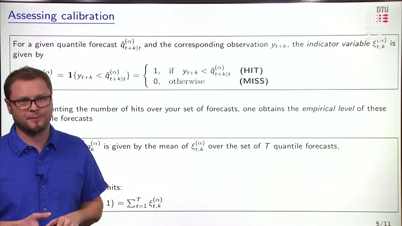




![Mar 5, 2025, Robert Huang [Caltech]](https://img.youtube.com/vi/88MMmA4KUr8/maxresdefault.jpg)