Make Multiple Dependent Dropdown Lists in Excel (Easiest Method)

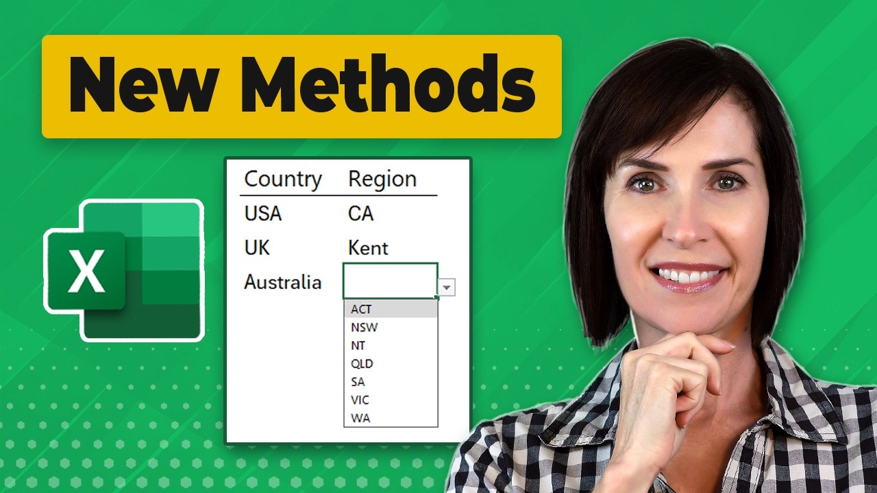
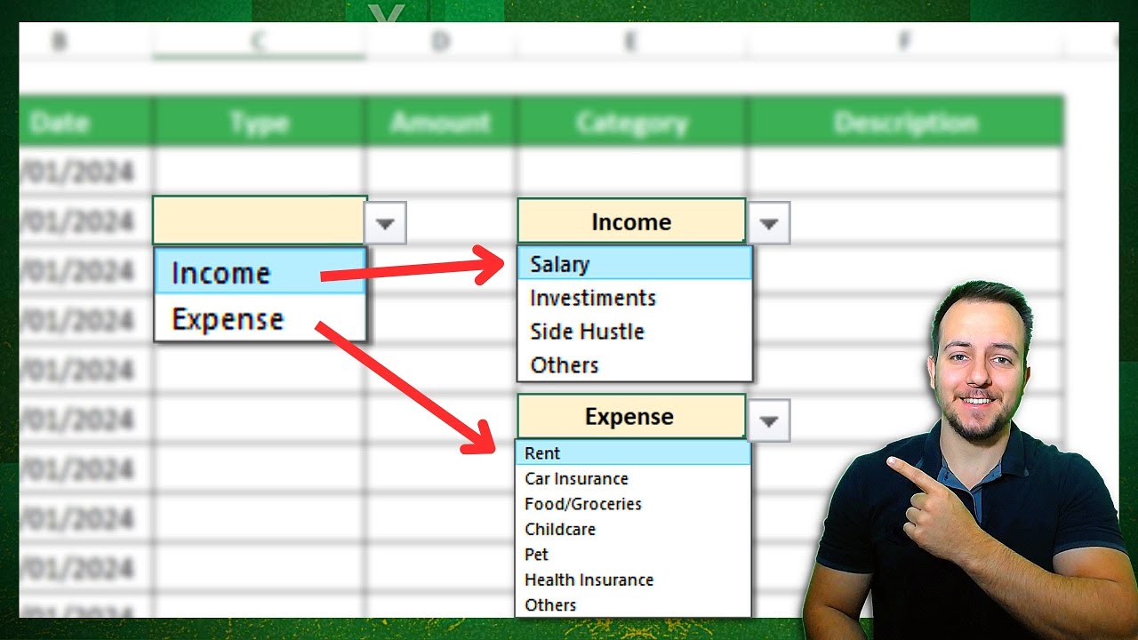
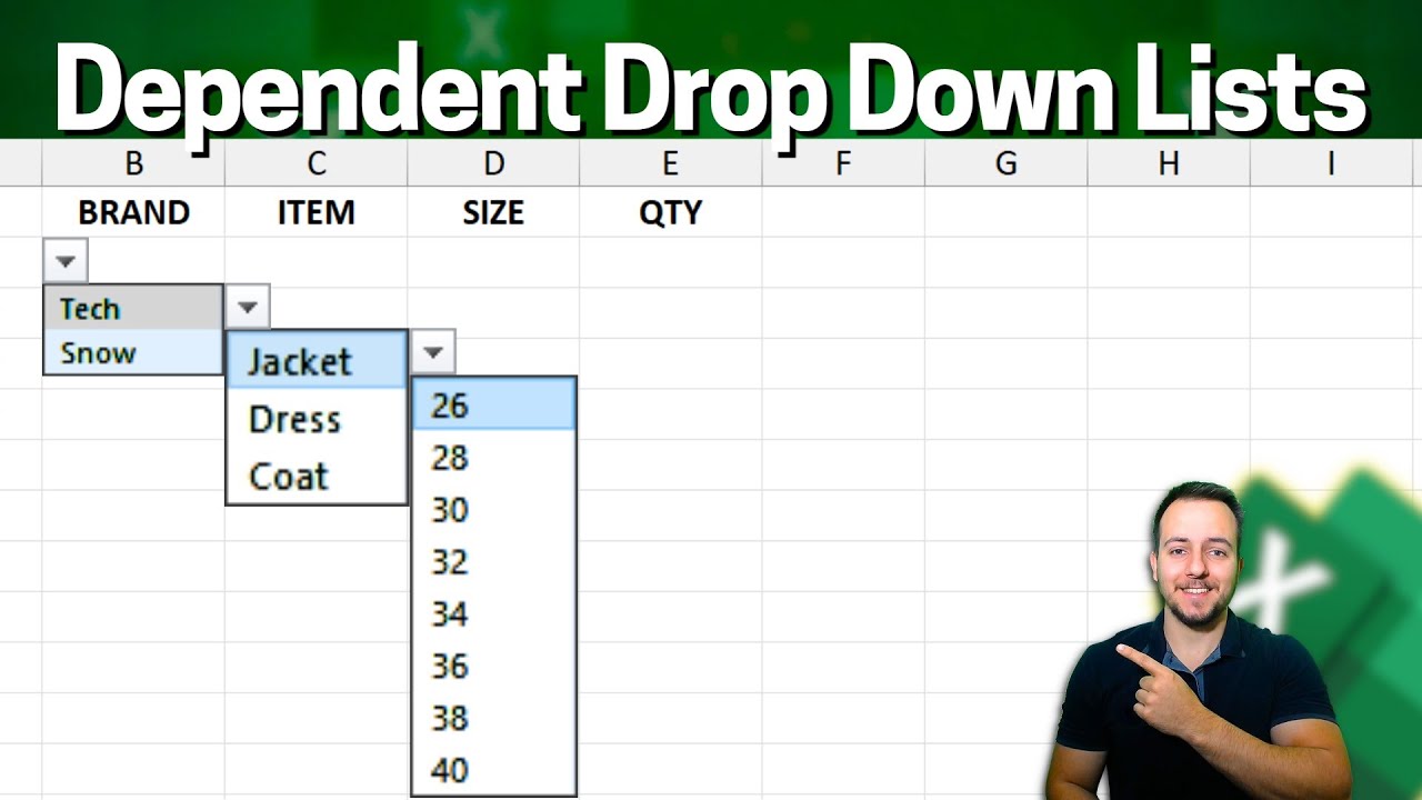
in this video you learn to make multiple dependent drop down lists in Excel and I know that sounds confusing so let me show you what I mean by choosing a region here from the dropdown it's going to influence the countries that are available in the next dropdown for example if we choose Europe we're only going to see the European countries and if we change this to Asia it's only the Asian countries that are there and the same idea goes with the city after that once we understand dependent dropdowns we create an advanced scenario where answers

autop populate depending on your choice and we'll even have a red error check in the case that we have a region that's in Europe and a country that's in Asia which obviously doesn't make sense and all of this is actually surprisingly easy to make let's take a look first up suppose we work for a large company and they have all of these offices available in these regions and we're going to go over four examples that are progressively harder which you can download for free in the video description to follow along so over here for the

region we first need to create a dropdown for all the region options and this is quite easy we just go over to data and click on data validation from here you'll get this popup that we want a list and that list is simply going to be all of the different regions so from E2 all the way to H2 and click on okay now you can see that we have all of the regions available let's say I just click on Asia and if you want to copy this down you can simply just drag it along like

so and you can see we get Asia but for now I'm going to delete all of these options and just stay with the top one now based on that we want to see all of the countries that are in Asia as a drop down so it would be these three over here and then when I change this to Europe it should change to this list right here for that the formula that we'll be using is a simple x lookup so it's equals x lookup hit the tab key and the look at Value is we're looking

for Europe comma and we're looking for Europe within this range up over here comma and if there's that much we want to see all of the corresponding countries which are these over here we can select the entire table there for all the countries and close that parenthesis so you can see right now for Europe we get all of this list and if I were to change this to say Asia then we get these three up here that's looking good and now we need to that whole X lookup inside of a data validation to make it

a drop down so I'm just going to delete it from here head over to data validation again we're going to want to have a list but this time around we'll put the X lookup inside so equals x lookup open up the parenthesis and we're looking for Asia so this cell right here B3 but we want it to move around so we're actually going to type it manually so it doesn't get those dollar signs comma and where can we find B3 we can find it in this region right here all of the region options comma and

then we can try to find the countries within this area right here which we selected before as well and you can see these are locked with the dollar signs so they don't move around but we want this one to stay Dynamic so it doesn't have any dollars click on okay there now we have the dropdown which if we click inside you can see we have Japan China and IND IND there if I switch this to let's say North America then all of a sudden my options dynamically change to US Canada in Mexico awesome so we've

Now set up a fully dependent drop down list with the region and the country but what if we also wanted to add another variable like the cities in this example that we can see here we have the countries listed and within each country maybe we have more than one office so you can see that we have three Offices here available for these cities and so we want to try to add that as well into our drop down conditions that's going to work in a very similar way so we'll click on data validation again and we're

going to want a list and that list is going to be an X lookup again so equals x lookup open up the parenthesis and now it's not region but country that we're looking at so it's going to be DC3 comma and we want to find that C3 within the range of countries this time it's vertical as opposed to horizontal Al like the previous example so we'll select all of the countries there comma and for the answers it's going to be all of the corresponding cities right next to them close the parenthesis and click on okay

now you can see we're under Asia Japan and the options are the three Japanese cities if I were to change this to let's say India then all of a sudden we get cities in India as three options nice in The Next Step we're going to be looking at how to autop populate so which shows certain answers depending on our choices but before that if you want to learn Excel fast and efficiently you can consider checking out our Excel for business and finance course here we teach everything we know about Excel specifically applied to real world

scenarios while we still cover theoretical lessons like formatting formulas and charts we also offer several case studies that simulate the type of work you might be assigned in your day-to-day ranging from Financial modeling to cleaning a data set and presenting some visual insights and if you get stuck along the way you can always ask us the course instructors any questions we also offer several other courses including SQL powerbi and much more so head over to the link in the description below to check that out the example so far don't tell us that much information it

would be nice to see alongside maybe the name of the country who the manager is how much that the country is made Etc and for that we'll take a look at this example where you can see we have not just the country but also we have some important let's say summary statistics to the side the idea is that whenever we choose a region from the dropdown and we select a specific country we want to see all of the corresponding answers there so right now this part isn't working so we need to add a data validation

again like we did before let me fast forward that great so now I have the drop down for Asia it's just giving me the Asian countries so that's looking good and right below that we want to make this dynamic as well to autop populate depending on our answer and we can do that with the X lookup mixed with another function so first we'll take a look at the X lookup here and we're looking for India comma we're looking for India within this whole range over here which is all of the countries that we have comma

and with that we want to get all of these answers so the revenue The Profit mark manager and the contact we can do those all in one go instead of having to write the formula four times simply by selecting the entire area there and close up parenthesis and hit enter you'll notice though that this doesn't look quite right and that's because the answers are horizontal as opposed to Vertical which is how we want them so we'll use this function called transpose which basically takes something that's horizontal and turns it into vertical or vice versa so

right here at the very beginning beginning of the X lookup we'll just put a transpose hit the top key there and simply close it at the end and now we can hit enter you can see all of the data now looks good we take a look at India you'll see that all of this is the right answer and if we change this to let's say Japan everything autop populates as well one problem you might have noticed with the current dropdown list is that the values sometimes stay fixed if we don't delete the country here but

we changed the region from Asia to Europe then this no longer makes any sense so to show that this is an error it would be nice to maybe cross out the value and even highlight it in Red so let's take a look at how to do that and it's going to combine a few functions firstly we would need to identify all of the countries that are within this region with a simple x lookup like we've done before so we're looking for all of the countries that are in the region of Europe so we're selecting Europe

within this range over here and we want it to spill out all of the returning countries in that region we'll close a parenthesis that's easy enough from here we want to see if any of these three match to the country if they don't then there's obviously a problem instead of getting these three values it would be good to have a true or a false depending on whether there is an error and for that we can put a count ifs here in front hit the toab key and the criteria range is fine as is comma and

we want to know if the criteria range is equals to the country of Japan or whichever country selected here we can close the parenthesis and hit enter so right now we get a zero meaning that it's false but if I were to change this to let's say France which is within that area within this list here then we get a one meaning it's true so now we have this error detector working correctly and we can use it inside our conditional for formatting what we'll do is copy this entire formula with contrl C there and hit

enter now we can go inside of the country cell under conditional formatting so go to the Home tab and click on conditional formatting we'll go all the way to the bottom where it says new rule here and within the popup we want to use a formula this is where we'll paste our formula and after that we need to say that if this is equals to zero that's when we have the error right it so that's when we want to change the formatting from what it currently has to something a bit different maybe we can go

ahead and add a strike through you can see in the preview what that looks like we cross it out we can also change the fill color to let's say a red and let's also change the font color to a white so it stands out there click on okay and click on okay again so you can see under the region of Europe France it's correct but if we were to change the region to let's say say Asia then all of a sudden France is incorrect we get that zero and you can see over here that it's

being crossed out obviously this part we don't need anymore as we copy pasted the formula but now you can see that it's fully error prooof awesome so you can see here conditional formatting is actually quite a flexible tool so you can learn how to use that even better with this video over here or by taking our Excel course over here hit the like and the Subscribe and I'll catch you in the next one