A Friendly Introduction to Machine Learning

hi and welcome to the machine learning P degree from udasi so we're going to talk about today is what is machine learning well this is the world and in the world we got humans and we got computers and one of the main differences between humans and computers is that humans learn from past experience whereas computers need to be told what to do they need to be programmed so they follow instructions now the question is can we get computers to learn from experience too and the answer is yes we can and that's precisely what machine learning

is of course for computer's fast experiences have a name it's called Data so in the next few minutes I'm going to show you a few examples in which we can teach the computer how to learn from previous data and most importantly I'm going to show you that these algorithms are actually pretty easy and that machine learning is really nothing to fear so let's go to the first example let's say we're St the housing market on our task is to predict the price of a house given its size so we have a small house that cost

$70,000 we have a big house that costs $160,000 and we'd like to estimate the price of this medium-sized house here so how do we do it well first put them in a grid where the xaxis represents the size of the house in square feet and the y axis represents the price of the, and so to help us out we have collected some previous data in the form of these blue dots these are other houses that we've looked at and we've recorded their prices with respect to their size so in this graph we can see that

the small house is priced at $70,000 and the big house is priced at $160,000 so now it's time for a small quiz what do you think is the best guess for the price of the medium house given this data would it be $80,000 $120,000 or $190,000 well to help us out we can see that these Blue Points kind of form a line so we can draw the line that best fits the data now on this line we can say that our best guess for the price of the house is this point over here which corresponds

to $120,000 so if you said $120,000 that is correct this method is known as linear regression now you may ask how do we find this line well let's look at a simple example this three points we're going to try to find the best line that fits through those three points obviously best line is subjective but we try to find a line that works well uh since we're teaching the computer how to do it computer can't really eyeball the line so have to get it to draw a random line and then see how bad this line

is so in order to see how bad the line is we calculate the error so we're going to for calculating the error look at the length of the distances from the line to the three points and we're going to Simply say that the error of this line is the sum of those three red lengths now what we're going to do is move the line around and see if we can reduce this error so let's say we move it in this direction and we calculate the error it's given by the yellow distances we add the up

and realize that we've increased the error so that's not a good direction to go let's try moving the other direction we move it here calculate the error now it's given by the sum of these three green distances and we see that the error is smaller so we actually reduced it so let's say we take that step we're a little closer to our solution if we continue doing this procedure several times we will always be decreasing the error and we'll finally arrive to A good solution in the form of this Line This General procedure is known

as gradient descent now in real life we don't want to deal with negative distances corresponding to a point being on one or the other side of the line so what we do to solve this is add the square of the distance from the point to the line instead and this procedure is called least squares so we can think of Granny the Santas trying to descend from a mountain this is our Mountain Mount aorist and this mountain the higher we are the larger error is so descending means reducing the error so what do we do when

to try to descend Mount well we look at our surroundings and try to figure out which way we can descend more for example here we can go in two directions to the right or to the left if we go to the left then we're going up which means our error is ascending this is equivalent to moving the line downwards and getting farther from the three points but if we go to the right instead then we're actually descending which means our error is decreasing this is equivalent to moving the line upwards and getting closer to the

three points so we decide to take a step towards the right then we can start this procedure again and again and again until we successfully descend from the mountain this is equivalent to reducing the error until we find its minimum value which gives us the best line fit so you can think of linear regression as a painter we look at your data and draw the best fitting line uh now this method is actually much stronger if the data doesn't form a line with a very very similar method we can draw a circle through it or

a parabola or even a higher degree curve for example the data here we can actually fit a cubic polinomial okay so let's move to the next example in this example we're going to build an email spam detection classifier so something that will tell us if an email is Spam or not and how do we do this we do this by looking at previous data the previous data is 100 emails that we've looked at already out of these 100 emails we have flagged 25 of them must spam and 75 of them must not spam now let's

try to think of features that spam emails may be likely to display and analyze these features so one feature could be containing the word cheap seems reasonable to think that an email containing the word cheap is likely to be spammed so let's analyze this claim we look for the word cheap in all these 100 emails and find that 20 out of spam ones and five out of the non-spam ones contain that word so we can forget about all the rest of the emails and focus only on the ones that contain the word cheap okay so

time for a quiz here's the question based on our data if an email contains the word cheap what is the probability of this email being spam is it 40% 60% or 80% well to help us out we can see that out of the 25 emails with the word cheap 20 of them are spam while five of them are not so this form an 8020 split so the correct answer was 80 if you said 80 you were correct so from analyzing this data we can conclude a rule the rule says if an email contains the word

cheap then we're going to say the probability of it being spam is 80% so we then associate this feature with the probability 80% and we're going to use it to flag future messages as spam or not spam we can also look at other features and try to find their Associated probability let's say we look at emails containing a spelling mistake and realize that the probability of an email containing a spelling mistake being spammed is 70% or let's say we look at emails that are missing a title and find out the probability of those being spam

is 95% etc etc so now when future emails come we can combine these features to guess if they're spam or not this algorithm is known as the naive Bas algorithm okay so now another example we are the app store or Google Play and our goal is to recommend apps to users so to each user we're going to try to recommend them the app that they are most likely to download we have gathered a table of data that we're going to use to make the rules and the table contains six people for each one of those

six people we have recorded their gender and their age and the app they downloaded so for example the first person is a 15-year-old female and she downloaded Pokémon go so here's a small quiz between gender and age which one seems like the more decisive feature for predicting what app will the users download well to help us out first let's look at gender if we split them by gender then the females downloaded Pokémon go on WhatsApp whereas the males downloaded Pokémon go on Snapchat so not much of a split here on the other hand if we

look at age we realize that everybody who's under 20 years old downloaded Pokémon go whereas everybody who is 20 or older didn't that's a nice split so the feature that best splits the data is age therefore if you said age that was correct so what we're going to do is we're going to add a question here the question is are you younger than 20 if yes then we'll recommend Pokémon go to you if not then we'll see so what happens if you're 20 or older then we look at the gender it seems like here if

you're a female you've downloaded WhatsApp whereas if you're a male you've downloaded Snapchat so we add another question here the question is are you female or male and if you're female we recommend WhatsApp and if you're male then we recommend Snapchat so what we end up here is with a decision tree and the decisions are given by the question we asks and this decision tree was built with the data and now whenever we have a user we can prove them through the decision tree and recommend them whatever app the tree suggests to recommend for example

you have a young person you recommend them Pokémon go if you have an older person you check their gender if it's a female you recommend them WhatApp and if it's a maale you recommend them Snapchat obviously there won't always be a tree that perfectly fits our data but in this class we're going to learn an algorithm which actually will help us find the best fitting tree to a table of data okay so let's go to the next example now let's say we're the Admissions Office at a university and we're trying to figure out which students

to admit we're going to admit them or reject them based on two pieces of information one is an entrance exam that we provide them the test and the other one is their grades from school so for example here we have student one with scores of nine out of 10 in the test and eight out of 10 in the grades and that student got accepted we also have student two with scores of three in the test and four in the grades and that student did not get accepted and then a new student comes in student three

this person has scores of seven and six and the question is should we accept them or not so let's first put them in a grid where the x-axis represents their score on the test and the y- axis represents their grades here we can see that student one would lie over here in the point with coordinates 98 since their scores were 9 and 8 and the student two would Li here in the point with coordinates 34 since the scores were three and four so in order to see if we should accept or reject student three we

should try to find a trend in that data so we look at the previous data in the form of all the students we've already accepted or rejected and it turns out that the previous data looks like this the green dots represents students that we've previously accepted and the red dots represent students that we've previously rejected so time for a quiz based on the previous data do we think student three gets accepted yes or no so to answer this question let's look closely at the data the red and green dots seem to be nicely separated by

a line and here's a line and most of the points over it are green and most of the points under it are red with some exceptions which makes sense since the students who got high scores are over the line and they got accepted and students who got low scores are under the line and they didn't get accepted so we're going to say that that line is going to be our model and now every time we get a new student we check their scores and plot them in this graph and if they end up over the

line we predict that they'll get accepted and if they end up below the line we predict that they'll get rejected so since students three has grades of seven and six a person will end up here at the point 76 which is over the line so we conclude that the students gets accepted so if you said yes that's the correct answer this method is known as logistic regression and now the question is how do we find this line that Best Cuts the data in two so let's look at a simple example this six points three green

three red and we're going to try to draw a line that best separates the green points from the red points and again a computer can't really eyeball the line so it can just start by drawing a random line like this one and given this line let's just randomly say that we label the region of the line is green and the region under the line as red so just like with linear regression we're going to try to see how bad this first line is and a measure of how bad the line is would be how many

points are we missing misclassifying we're going to call that number misclassified points the error this line for example misclassified two points one red and one green so we'll say that it has two errors so again like with linear regression what we'll do is move the line around and try to minimize the number of Errors using gradient descent so if we move the line a bit in this direction we can see that we start correctly classifying one of the points Bringing Down the number of Errors to one and if we move it a little more we

will correctly classify the other one of the points Bringing Down the number of Errors to zero in reality since we use calculus for a graded descent method it turns out that the number of Errors is not what we need to minimize but instead something that captures the number of Errors called The Log loss function and the idea behind the log loss function is that it's a function which assigns a large value to the misclassified points and a small value to the classified points okay so let's look more carefully at this model for accepting and rejecting

students let's say we have a student four who got nine in the test and one of the grades so this student gets accepted according to our model since they are over here on top of the line but that seems wrong since a student who got very low grades shouldn't get accepted no matter what their test score was so maybe it's to simplistic to think that this data can be separated by just one line right maybe the real data should look more like this where these students over here who got a low test score low grades

don't get accepted so now it seems like a line won't cut the data in two so what's the next thing after a line maybe a circle a circle could work maybe two lines that could work too actually it looks like that works better so let's go with that now the question is how do we find these two lines again we can do it using graded descent to minimize a similar log l function at before this is called a neural network now why is it called neural network well let's see we have this green area here

B about two lines this area can be constructed as an intersection namely the intersection between the Green area on top of one of the lines and the green area to the right of the other one of the lines so we're going to graph it like this we have two nodes each node is a line that separates the plane into two regions and from the two nodes we get the intersection which is the desired area the reason why this is called the neural network is because this mimics the behavior of the brain in the brain we

have the neurons which connect to each other and they either fire electricity or not they resemble the nodes in our graph which split the plane into regions and fire electricity if a given point belongs to one of those regions and won't fire if it doesn't so we can think of linear regression as a ninja will look at your data and cut it in half based on the labels and we can think of a neural network is a team of ninjas who will look at your data and cut it into regions based on the labels okay

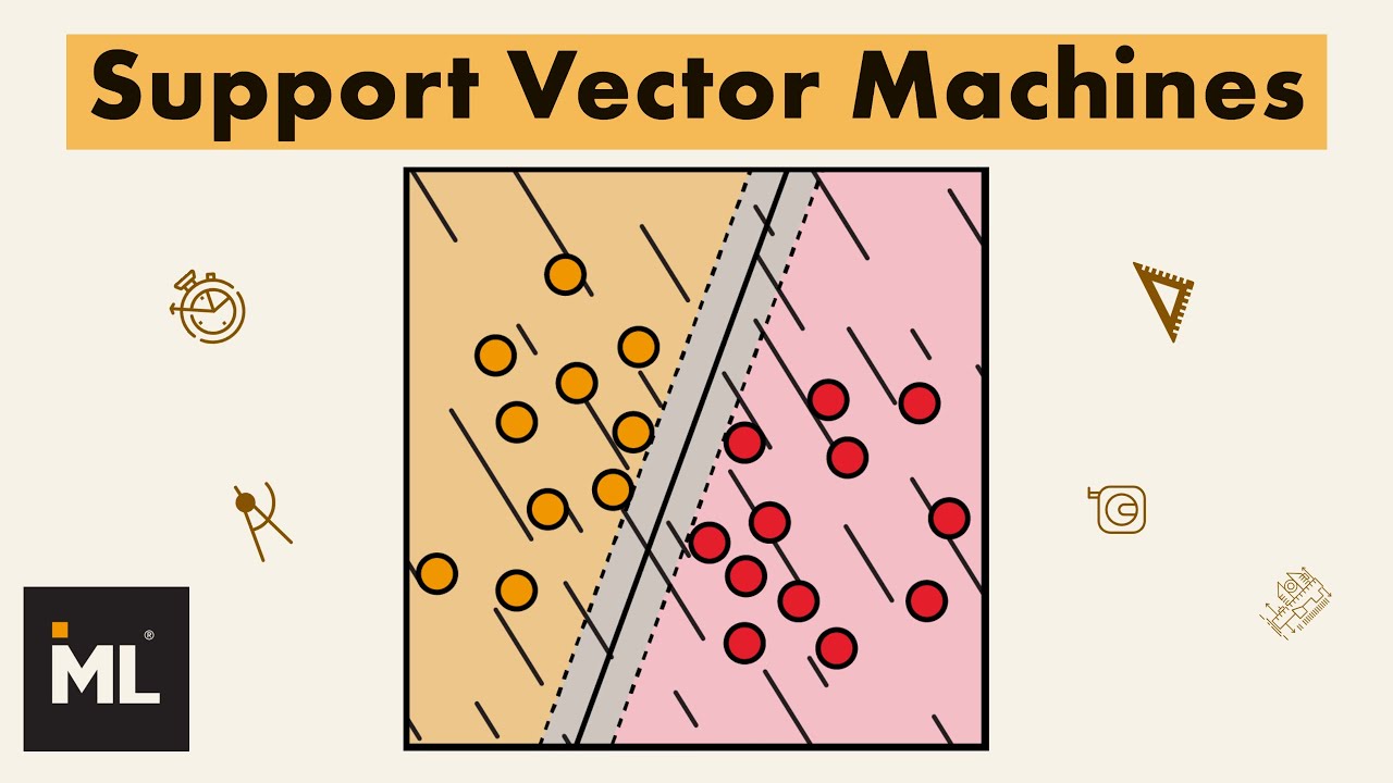
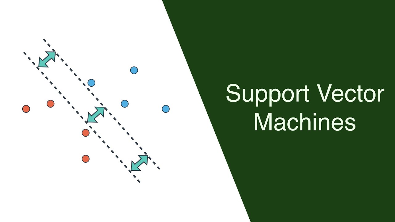
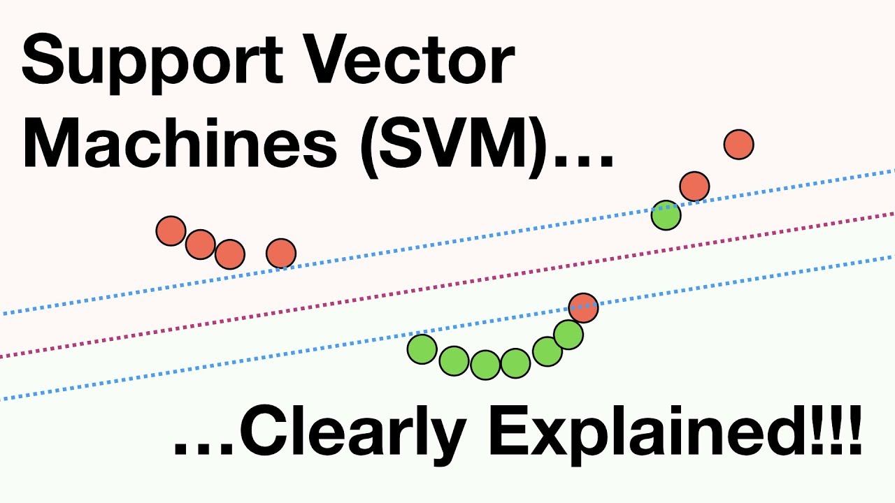
so let's dive a bit deeper into the art of splitting data into we can look at this points three green and three red and there seem to be many lines that can split them for example there is this yellow line and there is this purple line so quiz which of these two lines do we think cuts the data better the purple one or the yellow one well if we look at the yellow line it seems that it's close to failing it's too close to two of the points so if were to wiggle it a little

bit we would misclassify some of the points the purple one on the other hand seems to be nicely spaced and as far as we can from all the points so it seems like the best line is the purple one now the question is how do we find the purple line well the first observation is that we don't really need to worry about these points because they're too far from the boundary so we can forget about them and only focus on the points that are close and now what we're going to use is not grading descent

but we're going to use linear optimization to find the line that maximizes the distance from the boundary points this method is called a support Vector machine so you can think of support Vector machines as a surgeon who will see your data and cut it but before she will carefully look at what's the best way to separate the data into and then make the cut okay so now let's say we have these four points arranged like this and we want to split them seems like a line won't do the job since they're already over the line

and the red ones are on the sides and the green ones are in the middle so we need to think outside the box one way to think outside the box is to use a curve like this to split them another one is to actually think outside the plane and to think of the points is lying in a three-dimensional space so here are the points over the plane and here we add an extra axis the z-axis for the third dimension and if we can find a way to lift the two green points then we'd be able

to separate them with a plane so what seems like a better solution the curve over here or the plane over here well it turn out that these two are actually the same method don't worry if it seems confusing we'll get into a little bit more detail later this method is called the kernel trick and is very well used in support Vector machines so let's study one of them in more detail let's start with a curve trick so let's start by putting coordinates on the points this one is a 03 this one is 1 two this

one is 21 and this one is 3 0 and what we need is a way to separate the green points from the red points so the points coordinates are X Y then we need an equation on the variables X and Y that gives us large values for the green points and small values for the red points or vice versa so quiz which of the following equations could come to our rescue x + y the product x * y or X2 the first coordinate Square this is not an easy question so let's actually make a table

with the values of these equations on each of the four points so here's our table here we have the four points on the top row and now each of the other rows will be one of the functions so here's the sum x + y we fill in the first row the following way 0 + 3 is three 1 + 2 is 3 2 + 1 3 3 + 0 3 now for the second row we're going to get the products 0 * 3 is 0 1 * 2 is 2 2 * 1 is 2 and

3 * 0 is 0 and for the third row X squ is the first coordinate Square so 0 squar is 0o 1 s is 1 2 s is 4 and 3 S is 9 so let's let's think which one of these equations separates the green and the red points we look at the sum x + y and that gives us three at every value so it doesn't really separate the points we can look at X squar and that gives us different values for every point but we get 0 and N for the red values and

one and four for the green ones so this one also don't doesn't separate them but now we look at the product x * Y and that gives us zero for the red values and two for the green ones so that one seems to do the job right is a function that can tell them apart so that's the equation we're going to use you can see the products here and now for the red points X comma y we have that the product X yal 0 and for the green points we have that the product X Y

= 2 and what separates a zero and a two well a one so the equation x y = 1 will separate them and what is X Y = 1 it's the same as y = 1 overx and the graph for y = 1/x is precisely this hyperbola over here that is the curve we want it so that is the kernel trick now we can also see it in 3D here we have the 031 2 2 1 and 3 0 and we're going to consider them in three space so we're going to take the map that

takes the point x comma y to X comma y comma x * y so where does 03 go 03 goes to 0 comma 3 comma 0 since the product of 0 and three is zero 1 two goes to 1 comma 2 comma 2 so it goes all the way up since the third coordinate is the height the 21 also goes to 2 comma 1 comma 2 and the 3 0 goes to 3 comma 0 comma zero so there we go we can split them using a plane so you can think of a support Vector machine

Colonel method as a surgeon who is uh slightly confused trying to split some apples and oranges all of a sudden she comes up with a great idea the idea consists of moving the apples up and the oranges down and then successfully cutting a line through between them okay so let's move to the next example let's say we have a chain of pizza parlors and we want to put three of them in this city so we make a study and realize that the people who it Pizza the most living these locations and so we need to

know where where are the optimal places to put our three pizza parlors well it seems like the houses are nicely split into three groups the red the blue and the yellow so it would make sense to put one piece of parlor in each one of the three clusters but we're teaching a computer how to do this and a computer can just eyeball the three clusters we need an algorithm so here's one algorithm that will work let's start by choosing three random locations for the pizza parlor so they're here where the stars are located red blue

and yellow now it would make sense to say each house should go to the pizza parlor that is closest to it in that case we can look at the map like this where the yellow houses go to the yellow pizza parlor the blue houses go to the blue pizza parlor and the red houses go to the red pizza parlor but now look at the where the yellow houses are located it would make a lot of sense sense to move the yellow pizza parlor to the center of these houses same thing with the blue houses and

the red houses so let's do that let's move every piece of parlor to the center of the houses that it serves as follows but now look at these Blue Points they're a lot closer to the yellow pizza parlor than to the blue one so we might as well color them yellow and look at these red points they're closer to the blue Pizza po than to the red so let's color them blue and now let's do the step again let's send each pizza parlor to the center of the houses that it's serving in this way but

then again look at these red houses they're so much closer to the blue pizza parlor so let's turn them blue and then again let's move every Pizza poor to the center of the CES it serves and now we've reached an optimal solution so starting with random points and iterating this process helped us reach the best locations for the pizza parlors this algorithm is called K means clustering but now let's just say we don't want to specify the number of clusters to begin with let's use a different way to group the houses so say they're arranged

like this it would make sense to say the following if two houses are are close they should be served by the same pizza parlor so if we go by this rule let's try to group the houses let's look at which houses are the closest to each other it's these two over here so we group them now what are the next two closest houses it's these two over here so we group them the next two closest houses are these two so again regroup them the next two closest houses are these two so we unite the groups

now the next two houses are here so we group them the next two close hour are here so we join the groups the next two Clos house are here but now let's just say that's too big so all we need to do is specify a distance and say this distance is too far When You Reach This distance stop clustering the houses and now we get our clusters this algorithm is called hierarchical clustering so congratulations in this video we've learned many of the main algorithms of machine learning we learn to find house prices using linear aggression

we learn to detect spam email using naive Bas we learn to recommand apps using decision trees we learned to create a model for an admissions office using logistic regression we learn how to improve them using neural networks and we learn how to improve it even more using support Vector machines and finally we learn how to locate pie of parlors around a city using clustering algorithms so many questions may arise in your head such as are there more algorithms the answer is yes uh which ones to use that's not easy given a data set how do

we know which algorithm to pick uh how to compare them and evaluate them given two algorithms how do you know which one is better than another one in a data set given the running time their accuracy uh Etc are there examples are their projects are their real life dat data that I can get my hands dirty with them the answer to all these questions and more are in the Udacity machine learning Nano degree so if this interests you you should take a look at it thank you