Build a Monthly Budgeting & Forecasting Model in Excel

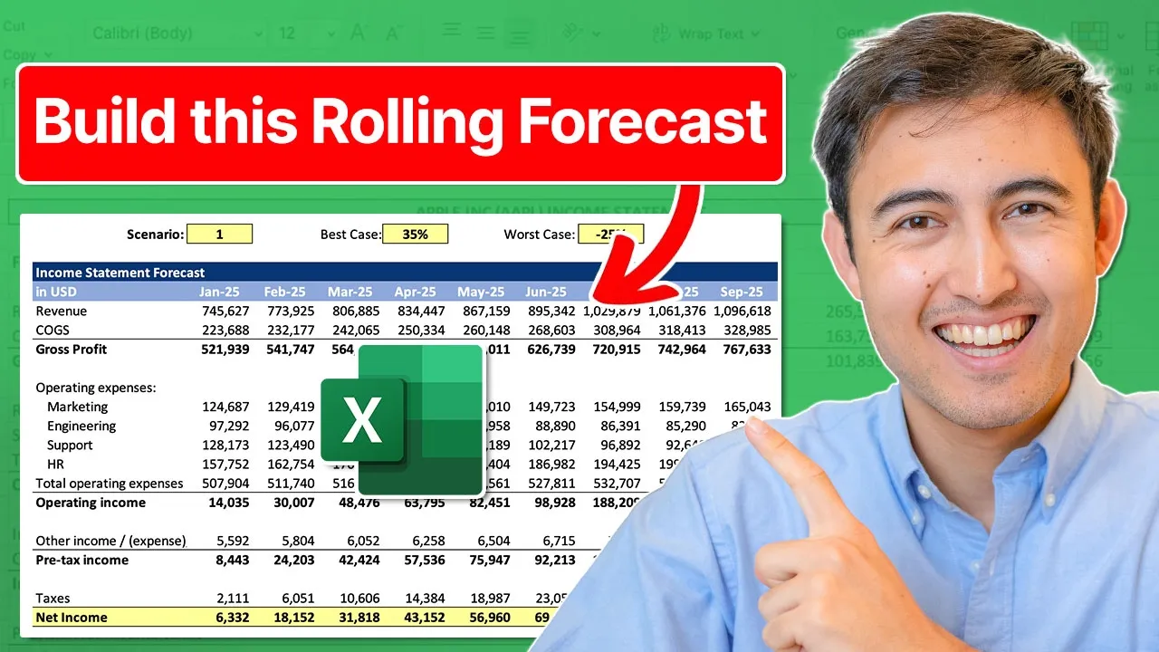
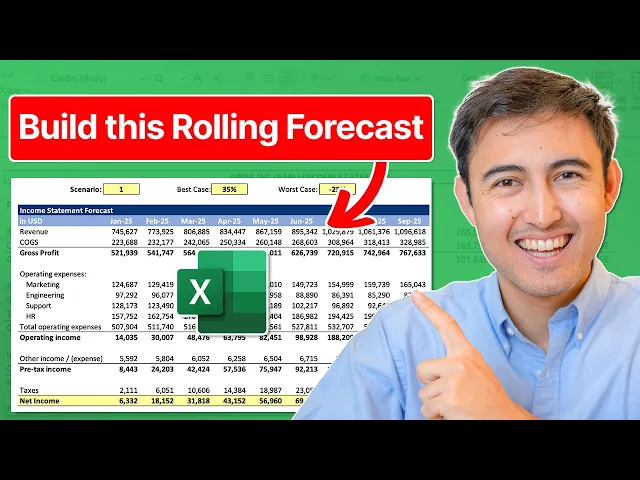
in this video we'll build a monthly budgeting and forecasting model in Excel first we'll take the actual operating expenses for each department second we'll forecast those going forward using excel's built-in forecasting tools thirdly we'll create different scenarios for these forecasts like a best case scenario and a worst case scenario and finally we'll build a full profit and loss statement to see how the forecast affects our profitability and because we'll make this model Dynamic we'll be able to see the impact of the different scenarios as well so let's get into it first up we have the

actual operating expenses in this sheet over here so you can see all of the different expenses by line and department and their description with the actual figures up top we have the start date so let's go ahead and Link that right in here like so and for all these other months that are also actual figures we just want to go to equals eate and that's the function we'll use we want this September and we want increments of one month so we'll just put a comma 1 in here close the parenthesis and this is October we

can move that all the way to December for our actual figures and you can download this Excel file completely for free in the video description to follow along once we have these actual figures well set up we can move on to the forecast sheet where you'll notice we have three different scenarios a best case a base case and a worst case down below and you can see that I have these x's on the left hand side so that I can navigate quickly just by pressing control down like so the idea is that with these three

different scenarios we'll be able to choose what we want for our forecast so first we just want to link all the three cases to our actual expenses as it doesn't really matter for the historical figures they're all going to be the same so I'm just going to press the equal sign and select it all the way from the account number once we have the first one selected I can press contrl C shift right arrow all the way to the column H and shift down arrow all the way to the bottom to here if we just

press crl + V to paste you'll notice we mess up the whole formatting so we'll press contrl Z instead and you'll notice down here under paste we have the paste special feature that's the same thing as going to control alt V once in here we just want to paste the formulas we don't want to paste anything else click on okay and you'll notice that all the data has now been copied correctly we want to do the same thing with all these other cases but now we can just copy from this best case part as they're

all going to be the same so shift down arrow shift right arrow and again not crl v as that messes it up but control old V and select formulas I'm going to do the same thing down over here a bit faster so I'm just going to link that to the account number and contrl C shift down arrow shift right arrow Control Alt V and paste the formulas awesome so we have the same data for our historical figures so now we're ready to do the forecasting and for this we're going to do it for a total

of 12 months let's add the date first so e dat it's a December comma 1 so plus one month shift right arrow and crlr there we want to do the same thing for this top part and the bottom part they're going to have the exact same dates for the different cases and let's first get started with this big Bas case now there's a few different ways to do a forecast the easiest way would probably be just take the average of all of this historical period but that doesn't work that well for outliers or if there's

a bit of a trend like the figures are going up the function we'll use here is the forecast. this function weighs the more recent data a bit more heavily than the older data and it also accounts for things like seasonality so if there's any Trends things like that so let's go ahead and select the target date that's the January 25 the thing is if we want to move this formula down we should probably make sure we have it well referenced so it doesn't move around so at the very start here in this I4 in that

14 part we want to add a dollar sign that's going to make sure we remain on row 14 even if we drag this down comma and the values are all of the historical values so all of these right here and as we move this to the right we want it to stay on the September Mark but keep expanding so what we can do is fix it at the column E mark with a dollar sign right here comma and finally for the timeline it's going to be this top part over here and again we're going to

put a dollar sign on the E other than this column e part we also want to add a dollar sign to the 14 and finally add another one over here under H to row 14 as well so it doesn't move now we're ready to drag this down so shift down arrow shift right arrow and press crlr for right and contrl D for down to check if these values look correct we can always go to the last one and you can see how it's extended everything all the way to the last value and it's looking at

December right now so that's looking correct we've just finished forecasting the base case and now we want to work on the upside or the best case and the worst case so let's take a look at those over here here we have the worst and the best but up top I'm just going to add a few more rows so control shift plus like so and let's call this the best and the other one is going to be the worst and the idea is that for the best case we can make an assumption like 30% increase and

the worst case is a 30% decrease something like that so with these assumptions we can calculate the very first one for the best case so that should save us some money these are expenses so we should have less in expenses so we can write equals to the base case multiplied by in parenthesis 1 minus the 30% so we're saying in our best case scenario we should have 30% Less in expenses close those parenthesis and hit enter we want to make sure this area is well locked so in the C2 we don't want that cell to

move around so we can press the F4 key there and hit enter now shift down arrow shift right arrow crlr and contrl D to drag it all the way down now we're ready to work on the worst case down below which should be very similar it's just going to be our base case multiplied by this time a worst case means there's going to be more expenses so we can do one plus that 30% so it's going to be 30% more in expenses again we want to make sure that C3 is well locked so we'll press

the F4 key there and hit enter now we'll do shift down arrow shift right arrow control d control R and we're ready now that we forecasted all three scenarios up top we added these two cells so let's quickly format them so first We'll add borders alt H ba there so that's the same thing as going up here and going to all borders and ALT HH to change the background color let's say I go for a yellowish color like that and the nice thing is that this should now be fully Dynamic so if I change this

top part to say 45% you'll see how all of the forecast figures are going to change so it's nice and easy for us to make any changes now we're ready to move on to the profit and loss statement where we'll put everything together but first if you want to learn more Advanced Financial modeling I'd recommend you check out our complete finance and valuation course here you'll learn all the essentials of accounting Finance valuation and financial modeling in Excel in the course first we'll cover financial statement analysis using Apple's real annual report as an example then

we'll get into Financial modeling through a three statement model on Apple after that we'll begin the valuation phase where you'll learn to do a discounted cash flow a comparable companies valuation and a prent transactions valuation on adobi looking at their real financial statements to eventually derive a valuation range lastly we'll show you how to present an investment thesis using a stock pitch format we also have a career track called the investment banker program which includes not just the finance and valuation course but also four other courses designed to make you stand out as an investment

banker so if you're interested in checking this out head over to the link in the description below all right back to the video so moving on to our income statement where we want to see how the forecast is going to affect our profitability and here you can see we have all the different line items and some assumptions that we'll look at later so first let's work on the operating expenses which is forecasted but you'll notice we have a lot of different line items that are duplicated like we have marketing a bunch of times same thing

with engineering and so what we can do here to list out all our unique ones is just use the unique function hit the top key there and under the array we're going to select all of the different departments we have and we should only see the unique ones here as is the case before we get into the numbers we also want to make sure that we have the month SEL Ed so it's going to be from January on shift right arrow and controlr for right you'll notice though as we get ready to put our different

operating expenses which of the forecasts should we use should it be the best case the base case or the worst case and right now if we select one it's actually not going to be dynamic which is not what we want so what we're missing here is what's known as the live case the idea is to be able to choose between these different cases with that so we we're going to press shift space to select the rows and control shift plus we're going to add a bunch of more rows here as we want to accommodate for

our live case let me just copy this part right here so I can copy all of the formatting all the way to December and we're just going to paste it up over here this is going to be our live case and don't worry with all these numbers breaking for now it's going to be equals to this part so all of our actuals should really be the same so I'm just going to drag that to the right like we showed you earlier Control Alt V and I'm only pasting the formulas you can see that side's looking

a lot better but for this part right here we want to delete these figures and make something Dynamic such that when we choose a scenario number one number two Etc from this top part we're going to be able to see the different scenarios from down below so for this we can use a formula called choose and the process is surprisingly easy all we need to do is select the index number so that's going to be the number one or whichever number it is that we choose press the F4 key there to lock that with the

dollar signs comma and the value number one this is where we select all of the cases let's say number one corresponds to our best case comma number two corresponds to our base comma and finally number three corresponds to our worst case you can see we have a lot more values we could put in here but we don't need them so we're just going to close the parenthesis and hit enter now I can press shift down arrow shift right arrow again contrl D and crlr and whenever we change the operating scenario here to let's say number

two all of these figures should change automatically and we're ready to now put it all in here as we're simply going to link the live case there's a few different formulas we could use but we're just going to go with a sum ifs the sum range are going to be all of the marketing expenses which we can find over here in our live case so that's going to be all of this part right here and then we're going to filter it by marketing only but we want to make sure that we lock the relevant areas

and this part is actually quite tricky so make sure you pay attention over here we're going to First Lock only the rows so this way just in front of the S and in front of the 14 with the dollar signs that means that the numbers are not going to move up and down but we can move them sideways across the different months comma the criteria range number one is all of the different departments so we have them here selected and we can lock that fully with the F4 key we don't want this to move sideways

or up and down comma and criteria number one is that it has to be equals to this one right here which is marketing you can't quite see it there but it's income statement b11 and we want that to stay fixed at that column B so it doesn't move to the side either now we're ready to close this with a parenthesis hit enter and shift down arrow shift right arrow controlr and contrl D awesome we can now calculate the total operating expenses with alt equals and shift right arrow controlr because we've made this fully Dynamic when

we change the scenario to number one let's say or number three you can see all the figures are updating we've done the operating expenses and we can now move on to the revenue line up over here are going to be our Revenue figures but we need some assumptions for these like what's going to be our price or our unit sold we can calculate all that down over here first we've got what's known as the customer acquisition cost so how much does it cost us to acquire a customer let's suppose I put something like 30 bucks

and we charge for a physical product that we sell let's say 279 we can then drag that to the side with crlr and along the way maybe we become better at marketing we are more efficient so we could switch that number to say 25 and take that all the way to the side and maybe due to inflation we increase the prices a bit to$ 299 knowing that we can calculate our unit sold which is going to be our total marketing spend so however much we've spent a marketing right here divided by our cost of acquisition

hit enter here and so it's saying we've sold 3,000 units then to calculate our Revenue it's just the unit sold multiplied by the price now we're ready to drag that to the right with crlr and we can link it to the top Revenue line so equals to this figure right here hit enter shift right and controlr for the cost of good sold here we can also make an assumption so that's a cost for us to produce the physical product that we're selling so let's suppose that that's 30% of our revenue and you might have noticed

by now some figures are in blue others are in Black essentially the blue ones are hardcoded values or values that we've made an assumption for while the black ones are ones that we have calculations for this way we know what we can manually type and change like this value here I could put a 31 but this part we really shouldn't be changing or it's going to mess up everything else so we have this cogs assumption and we can multiply the revenue times the 30% here to get that side all fixed contrl R to Dr to

the right and now we can finish up this part so that's equals to the CX here and the gross profit is the revenue minus the cost of good sold now shift right arrow and contrl R we can also get the total operating income here which is just the gross profit minus our total operating expenses shift right and controlr now let's work on this other come or expense part which is this part right here on the bottom let's suppose that's just 2.5% of cost of good soul will make that assumption that's equals to this figure multiplied

by our cost of good sold assumption so it's this one over here shift right and controlr finally for the tax rate let's say that's around 25% that seems fairly standard so right here we're going to do equals to this figure that we just calculated and our pre-tax income is the operating income minus our other income or expense shift right and control R finally for the taxes that's our pre-tax income multiplied by that 25% over here hit enter again shift right arrow controlr and here I've made a mistake because I've only left the 25% once here

in the front so we're going to need to lock that part with the F4 key there and now we should drag it to the right and control R so the net income is equals to the pre-tax income minus any taxes and we have the full pnl press crlr and it's all Dynamic now so I can change it to scenario number one or number three but you might have noticed something a bit strange if you've been paying careful attention here and it's that when we have the scenario number one which in theory is our best case

scenario we have a lower profitability or a lower net income then in scenario number three which is our worst case so that's not good and in fact when we take a look down over here we assume that the revenue is tied with our marketing so with our cost of acquisition as you might recall from here that's why in the forecast we should change the marketing expenses and how those are working right now in our best case they're going down by 30% but maybe we should switch that to going up by 30% just for the marketing

side so here we're going to change that to a plus sign hit enter so these two right here they should have updated controlr and contrl d and down over here as well for our worst case instead of spending more in marketing we can switch that to spending less by putting a minus sign in front so that's just going to be for marketing in the form of paid ads and influencers here so contrl d contrl r and now if we check our income statement again we go scenario number one it's a lot higher in profit and

scenario number three is a lot lower that said if we have a negative pre-tax income we shouldn't have to pay anything in taxes so we can create an if statement in here that's going to say that if this figure that c19 is greater than zero comma then we should get taxed but if it's less than zero there's nothing for us to get tuxed on so we can just put a zero in here close up parenthesis and just drag that to the right so contrl R so it's all zero because our pre-tax income is negative but

if we have a more positive one like this case here you can see that we are in the tax one final bonus trick we can add is in the operating expenses scenarios here if we change this to a zero or a number that doesn't exist we get this completely broken model so we should protect this by adding a data validation here we can go to the data Tab and click on this button to the side we want to select a list and we really only want people to put three different values so 1A 2 or

three click on okay and now if someone tries to put a four in here you'll notice they're not able to do that and it says to retry so I can put a two I can put a three or any other number only from this drop down once you've built the model it's very common to do a sensitivity analysis to see how all the different assumptions impact profitability you can learn how to do that with this video over here or by taking our finance and valuation course over here hit that like and that subscribe and I'll

catch you in the next one