today we're going to cover our first reinforcement learning algorithm which is called policy gradient now policy gradients are in some ways kind of the simplest reinforcement learning algorithm in that they directly attempt to differentiate the reinforced learning objective and then perform gradient descent on the policy parameters to make the policy better so to start with let's recap the objective function for reinforcement learning from last time reinforcement learning we have a policy which we're going to call pi that policy has parameters theta and the policy defines a distribution over actions a condition in either the state's
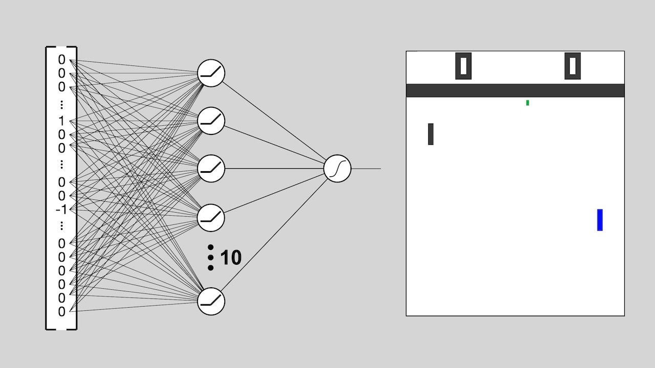
s or the observations o and i'll come back to the partially observed case later in the lecture but for now we'll just work on policies that are conditioned on states if the policy is represented for example by a deep neural network then theta denotes the parameters of the policy which are the weights in the neural network this network takes as input the state or observation and produces as output the action together the next state is determined by the transition probabilities which depend on the current state and the action produced by the policy and of course
then the next state sampled according to the transition probabilities is fed into the policy again to determine the next action and so on and so on this process can be used as we saw last time to define a trajectory distribution the trajectory distribution is a probability distribution over a sequence of states and actions so it's a distribution over s1 comma a1 comma s2 a2 s3 a4 a3 s4 et cetera et cetera et cetera and i'm going to use the subscript theta when i write a trajectory distribution to emphasize that the trajectory distribution depends on the
policy parameters theta we can write it by the chain rule of probability as the product of the initial state distribution p of s1 and then a product over all time steps of the policy probability pi theta a t given s t times the transition probability p of s d plus 1 given s d a t and i will use tau as a notational shorthand whenever you see me write tau that just means s1 comma a1 comma s2 comma a2 comma s3 etc etc etc all the way out to s capital t a capital t now
crucially when we develop model free reinforcement learning algorithms of the sort that we'll cover in today's lecture and the subsequent few lectures we typically do not assume that we know the transition probabilities p of s d plus 1 given s d a t nor the initial state probability p of s1 we just assume that we can interact with the real world which effectively samples from those distributions as we saw in the last lecture the objective of reinforcement learning can be written out as an expectation under this trajectory distribution so we have our reward function r
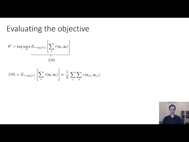
of s d comma a t and we would like to take the expected value of the sum of the reward under the trajectory where the trajectories are distributed according to p theta of tau and then we would like to find the parameters theta that maximizes expectation now as we saw in the last lecture we can push the sum out of the expectation by linearity of expectation and then express the expectation as an expectation of our marginal and this allows us to define both a finite horizon version of the rl objective and an infinite horizon version
in today's lecture we will focus on the finite horizon version although it's quite possible to extend policy gradients to the infinite horizon setting by using value functions which we will discuss next time so for now we'll stick to the finite horizon version where the sum is inside of the expectation but we'll come back to the other version later on okay before we talk about how we optimize the reinforcement learning objective let's first talk about how we can evaluate it so if we have a policy with parameters theta can we figure out approximately what is the
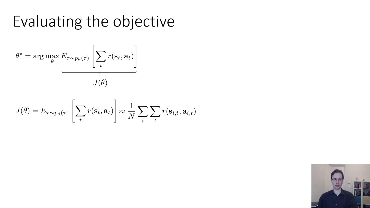
value of the reinforcement learning objective and i'm going to use j of theta as notational shorthand for the expected value under p theta of tau of the sum of the rewards so if you see me write j theta i'm just referring this whole expectation so if we don't know p of s1 and we don't know p s t plus one given st how can we estimate j of theta so take a moment to think about this since we assume that we can run our policy in the real world which amounts to sampling from the initial
state distribution and the transition probabilities we can evaluate j of theta approximately by simply making rollouts from our policy we run our policy in the real world n times to collect n sampled trajectories and if you see me write tau subscript i that refers to the ith sample if you see me write s subscript i comma t that refers to time step t in the ith sample having generated these samples from d theta of tau we can get an unbiased estimate for the expected value of the total reward simply by summing up the rewards along
each sample trajectory and then averaging the rewards over the sample trajectory as per this equation and the more samples we generate the larger n is the more accurate will be our estimate of this expected value so visually you can think of it like this we'll generate some number of trajectories in this case three for each trajectory we'll sum up their rewards to see which ones are good and which ones are bad and then we'll average them together and this will give us an estimate of j of theta now of course in reality we don't just
want to estimate the objective we actually want to improve it so to improve the objective we need to come up with a way to estimate its derivative and crucially the estimate of the derivative itself needs to be feasible without knowing the initial state probability nor the transition probability so again for rotational convenience i'm going to use p theta of tau to denote the structure distribution and i'll actually use r of tau as shorthand for the sum of the rewards over all the time steps in the trajectory table this will make the notation in the derivation
that follows a little bit easier to parse now if i have an expected value i can expand that expected value as a sum over for discrete variables or an integral for continuous variables of the product between the probability and the value so the expected value of r of tau under b theta of tau is equal to the integral over all trajectories of p theta of tau times r of tau and now we can start working on our derivative so our goal is to compute the derivative or gradient of j of theta with respect to theta
and since the refreshing differentiation operator is linear we can push it inside the integral so this derivative is equal to the integral over all trajectories of grad theta p theta tau times r of tau and i'll often say in this lecture just p of tau usually when i say p of tau i just mean p theta of tau okay so now so far this doesn't actually give us a practical way to evaluate the policy gradient because grad theta p of tau requires differentiating through the unknown initial state distribution and the unknown transition probabilities but there's
a very useful identity that will allow us to rewrite this equation in a way that we can evaluate using only samples much like how we evaluated the objective value so the convenient identity that we will use and this is basically the only piece of mathematical cleverness in this whole derivation is that if we have an equation like this if we have p of tau times grad log p of tau we can write it as p of tau times grad p of tau over p of tau this follows directly from simply the equation for the derivative
of a logarithm so if you open a calculus textbook and look up the derivative for uh you know d dx of log x you'll find that's that is basically equal to dx over x right so that means that grad log p is grad p over p but now you'll see that we have a p in the denominator and we have a p in the numerator so these cancel out which means that this is equal to grad p and what we're going to do is we're going to apply this identity in reverse so we have a
grad p here and we'll substitute the left hand side of this identity to rewrite it as p times grad log p and now you'll notice that we have an integral overall trajectories of p of tau times some quantity which means that we can also write it as an expectation we can write it as an expected value under p of tau of grad log p tau times r of tau and this suggests that we might be on the right track because when we have an expectation we can evaluate those expectations using samples we're not done yet
because we still have this grad log p tau term so let's work on that a little bit let's uh bring up again our equation for the trajectory distribution so p of tau which is just another way of writing p of s1 comma a1 comma s2 etc is equal to this product that we saw before if we take the logarithm of both sides the logarithm of a product is the sum of logarithms which means that we can write log p of tau as the sum log p of s1 plus a summation from t equals one to
capital t of the log probabilities under the policy plus the log transition probabilities and now we'll substitute this whole thing in for grad log pi i start grad log p and we're taking the derivative of this with respect to theta now the derivative with respect to theta of log p of s1 is just zero because p of s1 does not depend on theta and the derivative with respect to theta of log p of s t plus 1 given s t a t is also 0 because the transition probabilities also do not depend on theta so
that means that after the simplification the only terms that are left are the log pi theta a t given s t terms which are actually the only terms that we can evaluate because we know the form of the policy and we can evaluate the policy's own log probabilities so collecting all the terms that remain and expanding out our notation we're left with this equation for the policy gradient the gradient with respect to theta of j of theta is equal to the expectation under p theta of tau of the sum from t equals 1 to capital
t of grad theta log pi theta 80 given st times the sum of the rewards and now everything inside this expectation is no because we have access to the policy pi and we can evaluate the reward for all of our samples all of the unknown terms the initial state distribution and the transition probabilities occur only in the distribution under which the expectation is taken so that means that if we want to evaluate the policy gradient we can use the same trick that we use to evaluate the objective value we can simply run our policy which
will generate samples from p theta of tau sum up their rewards to determine which trajectory is good or bad and then multiply those by the sum of grad log pies and then once we've estimated the gradient in this way we can improve our policy simply by taking a step of gradient descent taking the old policy parameters and adding to them the policy gradient multiplied by a learning rate alpha if we think back to the anatomy of a reinforcement learning algorithm that we covered before the orange box here corresponds to the process of generating those samples
which are the ones that we're summing over the green box refers to summing up the rewards along each sample trajectory then we can calculate the policy gradient and the blue box corresponds to taking one step of gradient descent now this procedure gives us the basic policy gradient algorithm also known as the reinforce algorithm reinforces the acronym that was given by williams in in the 1990s to the first policy grading method which consists of three steps sample trajectories according to pi theta a given s by running the policy in the real world n times evaluate the
policy gradient as for this equation and then take a step of gradient descent so that's the basic policy rating algorithm what i've covered so far in this lecture basically gives you all the mathematical tools that you need to understand the basis the basics of policy gradients but if you try to actually implement the policy gradient as i've described so far it probably won't work very well so in the remainder of the lecture we'll discuss some of the intuition behind what policy gradients are doing and then discuss how to actually implement them so they work well
in practice which you will need to do for homework too