[Music] hey everyone and welcome back today we're going to explore simple linear regression and a little bit of a more serious context if you already know some of the basics about simple linear regression for example covariance correlation and the line of best fit and you probably don't know why they sort of work or what assumptions they're sort of built upon this is definitely going to be the video for you now if you've never explored simple linear regression i definitely highly recommend for example i'm looking at for example an introduction to bivariate data in my elementary statistics series first before diving into this because um in this approach we're actually going to be focusing a little bit more on the theoretical aspects behind simple linear regression uh some of its assumptions that make this model appropriate for bivariate data and a few other things along the way so with those things mentioned let's get started so as usual with bivariate data let's assume that we go out and ask people a series of two questions both of which have numerical responses and we're going to be associating them with a value x and a value y respectively and then we're going to be plotting them on a scatter plot and you're going to have this array of data points in r2 so as we should already know there should be a curve or more over a line that sort of approximates these data points to some degree of accuracy right so if this is a population data set then we can represent this line and which we're going to be representing as y hat to be equal to beta 0 plus beta 1 x where beta 0 and beta 1 are numbers and x of course is the predictor variable or the x variable that we're using to model the variable y so this line has a name and let's just name it here just in case you don't already know this is going to be our population line of best fit all right so of course the natural question that we need to start with is what do you mean so what do you mean by best because there are definitely different ways to define best fit so the most classical way that people define best in terms of linear regression is what is referred to as the least squares model or the least squares method or the least squares approach and what the least squares method does is well generally speaking all models is the goal is to find these numbers beta 0 and beta beta 1 that satisfy some criteria so the least squares method finds this beta 0 and beta 1 such that it minimizes a particular two-dimensional functional so the functional is sometimes represented as sse or error sum of squares some people represented ssr for some squared residuals and some people write it in functional notation as f of beta0 beta1 because this is definitely going to be a function that has beta0 and beta1 in it for which we seek to find so we define the sse or the sum of squared residuals as the sum from k is equal to 1 to m of the sum of the squared residuals of our data set so we have for example our response values y our associated predictor variables y hat x y hat k and then we square the difference which is called the squared residual so if we expand this because you may wonder well i thought this was a function of beta0 and beta1 well it is right because keep in mind beta0 and beta1 are in our predicted model so if we expand that out then we have f of beta0 beta1 is just the sum from k is equal to 1 to n of y k minus beta 0 plus beta 1 x k the quantity squared right so that is a multivariable function of beta0 and beta1 so if you give me some beta0 and beta1 it doesn't have to be the best ones you plug it into this equation sum across all your data points you're going to have a sum of squared residuals for that particular model now let's look at a couple things that you may visually pick up on so notice that this is in some sense a quadratic function right so you may think that okay well if this is the beta 0 axis and this is the beta 1 axis and this is for example the sse axis because i give you a beta0 and a beta 1 you're going to be able to give me an ssc if you have some data set right so if you graph this it should look like something like a parabola and if you sort of think that you're actually quite correct but of course this is not just a parabola it's a paraboloid so it's going to be a 3d surfaces so it's sort of looking like a bowl now a couple of things that if you're in for example an optimization class that you should be able to prove is the following so theorem one is the following this functional f or the sse is what we call a convex function so if you were to pick any two points inside of that bowl and connect them the line is going to be entirely inside of that bowl and it's a convex function on r2 that is the set of all pairs beta0 beta1 and since it is convex we can then find as a conjecture it has a unique minimum value i'm going to call it f star beta 0 beta 1 right so it has a minimum height so that height there that's going to be the minimum value for which the sse takes and that minimum value is generated by some point and a points beta0 and beta1 let's call it star that generates it right so in terms of this picture the beta0 star would be located somewhere right there and the beta 1 star would be located somewhere along that point right so there's a beta 0 star beta 1 star that generates the minimum value of f beta 0 beta 1 which we call the minimum value for which the sse can take all right so via this theorem which we're not going to prove this is more of optimization proof but definitely not super hard since it's a quadratic function since we know that the minimum value of f f exists and it's generated by this beta0 beta 1 that means there exists numbers beta 0 and beta 1 that we can find so the next question of course is what are they so theorem two which we will prove is that beta zero is actually equal to the mean values of the y minus beta one times the mean values of x now notice that we haven't actually found beta 1 but if we can find beta 1 solely on our x y data points and we have that beta 0 repre is represented as just a scaled version or a shifted version of beta 1 that means we can find beta0 and beta1 just from our data sets all right so how can we prove that this is actually the formula for the intercept so this is the intercept of the line of best fit via this least squares regression model right so let's give this a quick proof so since we seek to minimize things we're of course going to have to know something about differentiation and importantly minimization right so we take the derivative set it equal to zero solve since it's a minimum um we should be able to find that value so what i'm going to do is i'm going to take the partial derivative of a functional with respect to beta0 and i'm going to find the beta0 that minimizes that function so that's going to be equal to the partial derivative with respect to beta 0 of our functional the sum from k is equal to m of y k minus beta 0 minus beta 1 x k squared so keep in mind in terms of notation here y k and x k are both numbers beta 0 and beta 1 are variables okay and this is of course the a sum of things so keep in mind uh the derivative of the sum is the same as the sum of the derivatives so we can interchange those and then we can take the derivative of this quadratic function because we have the derivative of something squared so the derivative of something squared is going to be two times that thing times the derivative of the interior of that quadratic term so the derivative of y k is going to be zero because that is a constant the derivative of minus beta zero with respect to beta0 is just going to be equal to minus one and again xk is a number and beta 1 is a constant with respect to beta0 because this is a partial derivative not a total derivative so the partial derivative of any other variable aside from beta0 is going to be equal to zero because it's just a constant so that is our function and our goal is to find the value beta0 beta one that sets this equal to zero it's a convex function so whatever value generates that is going to be a minimum value so we don't have to do the second derivative test to uh verify that so notice that we have a negative 2 on the left hand side so we can divide both sides of this equation by negative 2 to eliminate those terms because that's still equal to zero on the right hand side so the next thing i want to do is a distribute this sum over those three terms so once i do that i'm going to have the sum from k is equal to m of y k minus beta 0 because that's just a number with respect to k at least the sum from k is 1 to n of 1 since there's nothing left there and then we have minus beta 1 times the sum from k is equal to m of xk all right and keep in mind that's going to be equal to 0. so you should know that if this is a population so technically that n should be a capital m but let's pretend that little n corresponds to the population size um that we have that that's just going to be equal to n times the population mean of y that's just another way of writing that and then if you add one to itself n times so one plus one plus one plus one n times that's just going to be equal to m and then over here we have the mean of x as usual so n times the mean of x there and that's going to be equal to 0. so notice that everything has n in it on the left-hand side and let's assume that our population is non-empty so n is greater than zero so we have no division by zero issues and we have that mu y is equal to beta zero actually mu y minus beta0 minus beta one mu x is equal to zero so keep in mind what we're solving for we're solving for beta zero so we're just gonna add beta zero to the right hand side and we have the beta 0 is equal to mu y minus beta 1 mu x which is the relation that we sought out to prove and that's how you can calculate the intercept of the linear regression line but keep in mind this depends on the slope of the linear regression line beta1 so now we need to be able to find a formula for beta1 that does not depend solely on beta0 and once we have that then we have the parameters associated to our least squares regression line now that we have an equation for the intercept of our linear regression 9 now we need to find a formula for the slope of our linear regression line and the proof is actually going to be a little bit more or it's going to follow the same steps or in the first few steps but later on it becomes a little bit more complicated so of course let's take this proof a little bit more slowly all right so what we're going to do is we're going to differentiate our function with respect to beta 1 instead of beta 0 this time so we're going to do the partial derivative of f with respect to beta 1.
so partial with respect to beta 1 of the sum from k sub 1 to n of y k minus beta 0 minus beta 1 x k the quantity squared so again we're taking the derivative of the sum which is the same as the sum of the derivatives and we're taking the derivative of something squared right so it's going to be 2 times something just like before so we're going to have 2 times the sum from k z1 to m of yk minus beta 0 minus beta 1 x k and then times the derivative of the inside so the derivative of y k is 0 because that's just a number and then we have the derivative of beta0 which is a constant as far as beta 1 is concerned because keep in mind we're not going to be using that identity yet right so let's pretend we do not know what beta0 is so that is independent of beta1 because we're not using that at this stage um so that goes away to zero and the derivative of negative beta one x k that's just gonna be equal to x k all right which is a number and then we're gonna be setting that equal to zero um we can divide both sides of this equation by 2 and 2 only we cannot divide by xk because xk could be equal to zero right there's nothing wrong with that um so that's the best we can do at least for now so once we have that let's just clean that up and let's actually distribute our xk inside of that bracket so we're going to have that the sum from k is equal to 1 to n is going to be taking the sum of x k y k minus beta 0 x k minus beta 1 x k the quantity squared and that's going to be equal to 0 and we want to of course find the value of beta0 and beta1 that makes this true all right so now what we're going to do is we're going to recall that formula for beta0 so keep in mind beta0 was found to be equal to mu y minus beta 1 mu x so we're going to be using that here so once we replace beta 0 which is located there with that expression then distribute that minus x k into that term we're going to get the following expression so we're going to have the sum from k sub 1 to capital m of x k y k minus mu y x k plus because we have a minus times a minus which is a plus so plus beta 1 mu x x k minus beta 1 x k squared is equal to 0. now what i want to do is i want to focus on all terms that do not have a beta 1 in it and i want to focus on all the terms with the beta ones in it so i'm going to be splitting this into three sums and treating of course beta 1 as a constant since we're taking the sum over k not beta 1. so once we have that we have the following things so we have the sum from k is 1 to n of x k minus mu y x k plus beta 1 times the sum from k is equal to 1 to capital m of mu x x k minus x k the quantity squared and that's of course equal to 0.
now before we move on with these algebraic things let's just recall a couple important tricks from basic statistics in particular the sum of y k minus mu y uh from k is equal to one to capital n we should be able to prove that that is equal to zero also you should be able to show the sum from k sub one to capital n of uh x k minus mu x that also is equal to zero so if we multiply both equations on the left by mu x we have that mu x is times that sum is going to be equal to zero as well so we have that the sum of mu x y k minus mu y mu x is equal to zero and the sum of mu x x k minus mu x squared that's also equal to zero so we're going to be adding zero to both of these expressions and doing some rearranging as well so in particular i'm going to be moving this term to the right hand side it's going to become negative but i'm actually going to be switching these two terms and factoring out a negative one to keep it positive on the right hand side so let's see if you can maybe do that on your own or maybe if you even if you can't just see if you can follow along here so once we perform that algebra we'll have the following thing so we have the sum from k sub 1 to capital m of x k y k minus mu y x k minus mu x times y k minus mu y so keep in mind this is equal to zero when we take the sum across it and then on the right hand side we're going to have beta 1 times the sum from k z1 to capital m and then we're going to have xk squared when we reverse it minus mu k xk when we reverse it and then minus mu x x k minus mu x and keep in mind again that this is equal to zero when we take the sum over it so using some basic factoring principles from precalculus you should be able to factor the interior of both of these summations so you should be able to show that this is actually the same as the sum from k is going to capital m of x k minus mu x y k minus mu y and the right hand side is the sum from k is equal to 1 to capital m of x k minus mu x the quantity squared now what i'm going to do is i'm going to divide both sides by capital m and you should recognize these formulas because on the left hand side that is just the covariance between x and y and the right hand side is just the population variance of the x values only so that means we have that the covariance for the population p is going to be equal to beta 1 times the variance of x right so once we have that then we have a formula for beta 1. so that means beta 1 is going to be equal to the covariance of the population between x and y divided by the variance of x so you should know another representation for the covariance formula you should know that that's actually the same as the correlation times the pi standard deviation of x and the standard deviation of y and if we look at that notice that we do have some simplifications there and we can write that just as uh correlation coefficient divided by the quotient of population standard deviations and therefore we have the beta one is equal to rho sigma y sigma x and we've already shown that beta0 is equal to mu y minus beta 1 mu x right so we have formulas for both of the parameters of our population line of best fit where these parameters are generated via the least squares approach which minimizes the sum of squared residuals the next theorem might not seem too exciting on the surface but it's a very very important result in order to prove other results that are actually quite very useful and it says this it says the beta 1 which is the slope of the simple linear regression line can be represented as a linear combination of the response values y that is if you're familiar with linear algebra this definition should be familiar there exist real numbers such that beta1 is equal to c1 y1 plus c2 y2 plus c3 y3 all the way down to cn ym so this proof is actually not too hard so let's see if we can give it a try so we already know a formula for beta 1. beta 1 again is just going to be equal to the covariance of the population divided by the variance of the x values so if we sort of expand the covariance and the variance and eliminate the ends what are we going to get so we're actually going to get the sum of x k minus mu mu x and then y k minus mu y and again that's the sum from k is equal to 1 to capital m and keep in mind that's also all over 1 over n and i'm actually not going to touch the variance formula i'm just going to leave that as sigma x squared and what i'm going to do now is i'm going to put the 1 over n and the sigma x term as a fraction under the x term only so what do i get when i have that so i'm going to have the sum from k is 1 to capital m of x k minus mu x over sigma x squared times n times y k minus mu y and you might be wondering well why would i want to do that so now what i'm actually going to do is i'm going to let ck be equal to xk minus mu x all over sigma x squared times n and my claim is that these cks are actually the cks we need for our linear combination all right so let's see if that actually is true so once i have that i'm going to have the beta 1 is equal to the sum from k is 1 to capital m of c k times y k minus mu y so it's almost a linear combination but it's not a linear combination of y k's the differences of y k to the y to the mean so what we're going to do is we're going to distribute those c k's across the y k's and that constant mu y and we're going to see some interesting things happen so we have that the sum from k is equal to n of c k y k so that's our linear combination that we want but that's not the only thing we have right because we have minus the sum from k is equal to 1 to capital m of c k times mu y agree so what exactly does that mean so let's bring back the definition of ck and we're actually going to see something very very neat here so we're going to have beta 1 is equal to the sum from k z1 to capital n of c k y k minus the sum from k is 1 to capital n that mu y is a constant so i can actually just factor that out and then we're going to have x k minus mu x all over sigma x squared times capital m keep in mind that sigma x squared and capital n have no dependence on k so technically i can factor them out outside of this fraction and i'm just going to have beta 1 is equal to the linear combination of our y values c k y k minus mu y divided by sigma x squared times m times the sum from k is 1 to m of x k minus mu x so do you remember what this term is equal to you should remember that that is actually equal to zero so zero times that is going to equal to zero and we're just left with our linear combination term which concludes the proof of that theorem right but again this theorem might not appear to be that interesting but this is definitely going to come in handy and of course keep in mind what these cks are the cks are going to be equal to xk minus the mean of those values divided by the variance and times the population size if this were to be a sample that would be x bar and n minus 1 in the bottom but this is the population perspective now i want to also mention since we're talking about linear combinations linear regression is that not all data sets are appropriate for linear models okay so there are a set of assumptions that we usually would like to be met in order to classify a data set as appropriate to fit a linear model so let me just briefly go through these assumptions and what they mean so the first is the conditional distribution must be associated to a normal distribution with some mean expected value of y given x and some variance variance of y given x value this is usually referred to as the normality assumption so what does this mean so if we have our x values and our y values we of course can sample across levels of each of our x's right so for example we can have some values there some values there some values there and some values there so what must be true is that the distribution of all those points from the population perspective needs to be normally distributed across those lines right and of course along each of them the means could be different the variances could be different but assumption one says that the distributions of those must be normal now the second assumption talks about some requirements about those means so the expected value of y given a particular value of x must be related to the x values in the following way there is that is there exist these numbers beta0 and beta1 such that the means are linear so if we look at the same exact picture but a different data set i guess and we sample for example across these values we would like for the means to be associated to a linear distribution so that should be there that should be there that should be there and those means should lie on a line that is there exists a beta0 and beta 1 such that those means fit exactly onto it from the population perspective so if this is a sample data then those means should lie approximately on the line right so that's pretty much definitely represents the linear assumption for this data set and the last main assumption is the variance of those normal distributions across these individual values because this is usually like x1 x2 x3 all the way down to like xm um each of these variances must be equal to some number which i'm going to call uh sigma squared some people also call it sigma squared y with respect to x and this is called the hamas elasticity assumption hamasa dasticity assumption and the second is called the linearity of means property now notice that this number sigma squared is not dependent on x the mean is dependent on x but sigma squared does not depend on x and just keep in mind notation that capital variable x that's going to be our little variable x so little x is a number capital x is a random variable right so when you choose a particular value of capital x the variance is equal to a number and that number or that constant is independent of the x value that you chose that is very very important and also i want you to also understand that sigma squared y given x is not definitely not the same as sigma squared y so this is the variance of all the y values this is the variance of all the y values across a particular level x a particular x not all of them a particular one so make sure you do not get them mixed up because they are definitely definitely different all right so sigma squared y and the sigma squared that we're using here are not the same thing okay now these three assumptions normality linearity and hamas elasticity are usually the basic assumptions some people also imply but i'm not going to label it as a fourth but this is usually always what we desire is the observations of yk should be independent of one another they should be independent of one another right as everything we do in statistics if you don't have independence then things become really really complex in terms of mathematics and also interpretation but usually we don't have a direct way of testing or even knowing that they are independent so we usually would like to assume that they are and that everything is well on the data analytics side right but that is usually another fourth property that we assume for appropriateness for fitting lines to data sets both in simple linear regression and auto also multiple linear regression later up to this point we've only assumed that we've been working with bivariate population data sets but usually we can't get the entire population to sample so we would have to sample from that population and get a subset of the population and then construct a linear regression line from that sample data set so can we still use the same formulas for the linear regression parameters not quite because they're estimates for the parameters for which we know are correct all right so before we get into what those approximations are going to be recall that x bar is an unbiased estimator for mu x which we write as the expected value of x bar is equal to mu x and similarly we have unbiased estimators for mu y the variance of x the variance of y and the population correlation coefficient all of which are our sample statistics that we already are familiar with so now what we want our goal is to approximate for example the vector beta 0 beta 1 with other numbers or random variables beta hat 0 and beta hat 1.
so keep in mind these are parameters they are numbers but these are statistics which are random variables now why are these random variables because they are based on random samples agreed so if we are going to be approximating beta0 with beta 0 hat and beta 1 with beta 1 hat that means we are approximating beta 0 which keep in mind was mu y minus beta 1 mu x we are approximating that with beta zero hat which is equal to for example y bar minus beta one hat x bar and we are approximating beta one which keep in mind was sig uh rho times sigma y over sigma x and we're going to be approximating that with beta 1 hat which is going to be r times s y all over sx now just because of the individuals statistic random variables are unbiased estimators of those particular parameters that does not necessarily imply that these linear combinations well not even linear because we're dividing in beta 1. 1 is also an unbiased estimator of those parameters right so here is a very important theorem that talks about this so one can actually prove that the expected value of beta 1 hat actually is beta 1 and the expected value of beta hat 0 actually is beta0 which of course is what we want now as usual with all of the statistics that we discussed up to this point although they are unbiased estimators they still have they still have some error associated to them some standard error associated to them associated to them right just like x bar just like x x squared just like r all those random variable approximations have standard error all right so here is the next theorem which i'm not going to prove but with all the things we've talked about up to this point you should be able to show that this is indeed true so one can show that the standard error for beta hat 1 is going to be approximately equal to 1 divided by sx times the square root of the air sum of squares all divided by m minus 2 m minus 1 and the standard error for beta hat 0 is going to be equal to the square root of sse divided by m minus 2 times the square root of 1 over m plus x bar the quantity squared all divided by m minus 1 times s x the quantity squared in the denominator definitely not the most beautiful of these things but you definitely should be able to show them if you're in the theoretical context of a class or maybe you really need to know where these formulas come from so you can change them for other models in the future just as a hint just use the variance operator on the definition of beta 1 hat and beta0 had do some algebraic manipulations do some tricks that we've discussed previously and then take the square root and that gives you the formula for the standard error all right so what about hypothesis testing so if the assumptions if the assumptions are met in particular normality linearity of means and hamas elasticity of the conditional variance and let's assume that we're interested in testing that the slope of a linear regression line is equal to some number let's call it beta 1 with a 0 up top then the associated test statistic is actually going to be a t test statistic which is going to be equal to our point estimate minus the claim value of the slope divided by that standard error beta hat one and if you're interested in testing that these intercept of the linear regression line is equal to some number called beta0 then that's also going to be associated to a t test statistic so one should be able to show that beta hat one and beta hat two are normal random variables that's actually where that linear combination theorem that we discussed previously actually has its highlight so the test statistic is going to be equal to the point estimate minus the claim value divided by the associated standard error and since they're associated to a t distribution they are going to have a degrees of freedom and the degrees of freedom is going to be equal to n minus 1 minus 1 or n minus 2 once you simplify that okay so those are our test statistics all right so another question that we need to answer so if the assumptions are met how to approximate how to approximate that hamas elasticity variance okay so here's a nice little theorem that sort of will help us with this so theorem seven so let s squared y given x be defined to be equal to the error sum of squares divided by n minus 2. then so that's going to be a random variable right because sse depends on a random sample so this s squared y given x is going to be a random variable then one should be able to show that the expected value of s squared y given x actually is equal to sigma squared y given x which is just equivalent way of writing that sigma squared that we had before now if you have been following me before you actually should know what the sse over n minus 2 is from anova test so what we're going to do is we're going to define it in the same exact way as the mean square error so we're going to call that sse divided by m minus 2 which is in expanded form m minus 1 minus 1.
and this 1 actually is going to change later but this is the number of predictor variables in your model later when we do multiple linear regression right now we just have one variable x but you could have x1 x2 x3 and so on so that's where that's going to change so that means this theorem can be represented in the perspective of mse so that means the expected value of mse the mean square error actually is equal to sigma squared so the mean square error is an unbiased estimator for the hamaston statisticity variance constant all right so let me go back to theorem six um because i mentioned that the standard errors were approximations but one can actually show the exact values in terms of the mean square error so one should be able to show that the variance of for example beta hat one is equal to that mse approximated variable divided by sx squared times m minus 1 and the variance of beta hat 0 is going to be equal to sigma squared times 1 plus n and then x bar squared divided by sx squared and minus 1. and of course this is the same as before because to get the standard error you're just going to be taking the square root of these variance terms and in case you do not know what sigma squared is you can approximate them with the mean square error for your sample take the square root and that gives you your standard error as usual so in case you already haven't figured it out especially by my notation of sse and mse regression and analysis of variance tests do share a various very close connection in particular we can define for example the sst the sse and the ssm which is actually where i choose these notations from solely from the regression perspective because in case you encountered with me the two-factor analysis of variance with interaction the computational things such as that are very very complicated but you can actually perform those same tests via regression and the computational things are actually a lot more easier to understand and represent so in the regression world what is going to be the sst so just like in the anova world the sst was equal to the variance of all the values which in this case is just going to be the variance of the y values times m minus 1. so from the sst the mst is going to be equal to the sst divided by its associated degrees of freedom which we know is just the same thing as the variance of the y values some people won't write the msd they'll just call the variance of y but when we get to building our anova table for regression it's nice to fill in all those little squares so that it looks complete so then we have our sse and sse actually has the same exact structure or similar structure as before but this is going to be equal to the sum from k is equal to 1 to m of y k minus y hat k the quantity squared so it's the sum of squared residuals and for the simple linear regression case you should be able to show that this is also equal to s y squared times m minus 1 times 1 minus the correlation coefficient squared or the coefficient of determination so once you have your sse then our msc which we've already defined is just going to be equal to the sse divided by the associated degrees of freedom m minus 2 which keep in mind is the same as m minus 1 minus 1.
very useful to define that later and then our ssm can be defined similarly to our regression our anova world this is going to be the sum from k sub 1 to n of the predicted values minus the associated average of all the y values and one should be able to show just like we did for anova that this is actually just going to be equal to the total sum of squares minus the error sum of squares ie sse plus ssm will always be equal to sst the only reason that i represent the formula for ssm here is because once we get into the multiple factor anova via regression we have to have a nice little formula to represent them so it's useful to keep this in mind here right now how many models do we have so notice that we only have one variable so the degrees of freedom for the ssm is just going to be one so in the simple linear regression msm is just going to be equal to ssm divided by 1 which is just going to be the ssm but later we're going to have more variables and we're going to divide by the number of variables that we have also one should be able to show via all these formulas so this is a very very nice calculation to perform but it's also very very neat as well and it's going to come in handy later is that the coefficient of determination or the squared correlation coefficient is actually equal to ssm divided by sst so since we know that the sum of sse and ssm is sst we can actually represent this as sst minus sse divided by sst and then we can decompose that fraction and write this as 1 minus sse all over sst and that's an alternative way of writing the coefficient of determination and regression yeah it might not be very exciting to you now but later this perspective is going to be very very useful in the multiple linear regression approach now that we have all these anova-like metrics now what we're going to do is construct an anova table for our regression model so it's going to have the same exact setup just like the anova test so we're going to have our variation source as our first column we're going to have our degrees of freedom for our second column we're going to have the sum of squares as our third column and then we're going to have our mean squares for our fourth column so we have our model we have our residuals and then we have the total right so though that is our anova table setup so for the simple linear regression model the degrees of freedom for the model is going to be one that's how many variables we have um the total is going to be m minus 1 which we already know and we should know that that's going to be equal to m minus 1 minus 1 which is n minus 2.