ANOVA: One-way analysis of variance

hi and welcome to zed statistics today we're going to deal with the concept of Anova or analysis of variance uh it's a very important Concept in statistics and it pops up all over the place uh in particular you might recognize it from your studies of regression if you've previously dealt with that topic uh but here we're actually dealing with it in a more pure form we're dealing with it as it applies to a single variable and and this is what we call One Way Anova if you're keen on seeing how Anova applies to regression I'll

put up a link right here that you can follow to my series of regression videos and this will be the one that will deal with Anova as it applies to regression but let's get on with Anova in a one-way context so first step is to consider what variance actually is now hopefully you've seen this formula before uh but if we look at it it's just the deviation from the mean of each observation so observation X we calculate its deviation from the mean minus xar and then we Square it and add them all together that's what

that sum symol means um and so we're essentially finding some measure of the spread of the data now don't worry too much about the N minus one for the moment because realistically we're only at this stage interested in that numerator the sum of squares which we're going to call SST or total sum of squares sum of squares total so in a sense you can call it the analysis of sum of squares as opposed to the analysis of variance so as an exercise I'm going to get you to try and find the total sum of squares

for the following two samples uh here's a and b and what I want you to do is try to use this formula here and find that figure the SST for both of these two samples it's really quite crucial to get your head around what SST represents so I'd recommend pausing the video and seeing if you can come up with the answers so with that done the first step is to find the means of these two samples which is simple enough the mean of a is three and the mean of B is n now the SST

for a using this formula I'll just go through it very very quickly we take each of these observations in turn so we go two and then we subtract three we subtract the mean and then Square 2 - 3 is -1 and we Square It 2 again - 3 is -1 and we Square it Etc and then we get a sum of squared total or total sum of squares of six and if you tried it with B you should have got 42 and you can see that the larger the SST the greater the spread of the

data and that's evident when you look at A and B respectively B clearly has a higher spread or variance and that comes out in the SST let's not forget this is the numerator of the variance equation anyway so let's have a look at what oneway Anova actually is we're going to use this example now um which is theoretical stats test where there were nine students and you can see the top score was nine perhaps out of 10 and the bottom score was one and there was lots of scores in between um the first step is

always to calculate this total sum of squares that is the variance that's the variation I should say that we're actually dealing with which we're going to try to explain and the total sum of squares in this case is 42 which you can try yourself but perhaps you'll just believe me now let's presume that there were three different streams or classes and you can see that in one stream we had the person that scored one the person that scored five and someone that scored nine in that stream stream two we had a 456 and stream was

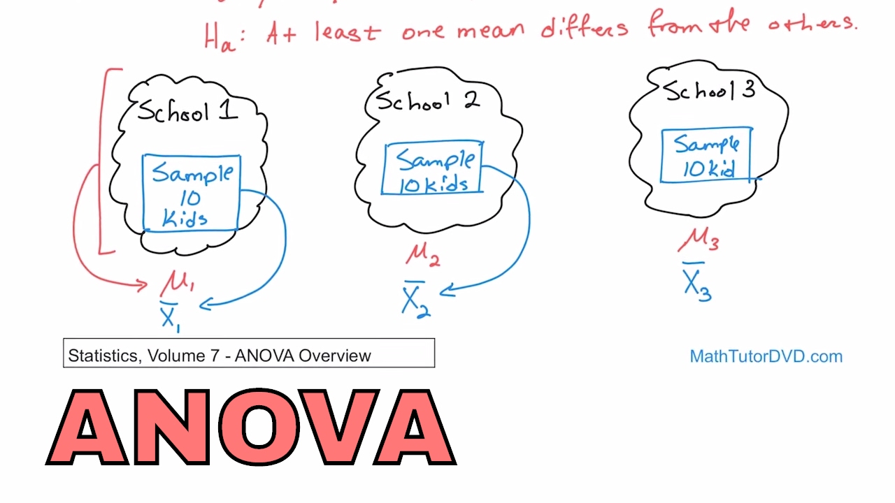
357 now the question is and this is what One Way Anova asks is is there a difference between the streams can we say that stream one did better or worse than stream two or stream 3 Etc so how do we do it here's a little plot to show you the three streams and I basically just put the means they're the dots in the middle and then the maximum and minimum at the top and bottom you can see here that the mean of each stream is actually very similar in fact it's exactly the same the mean

of stream one is five the mean of stream two is five and three is also five so if you ask the question is there a difference between the three streams you could probably say no straight away in fact you could definitely say no straight away so let's just see how one way a Nova goes about answering that question what it does is it splits that total sum of squares into two components which is the sum of squares within groups and the sum of squares between groups now they've got slightly different formula but I'm not going

to really deal with the formula because I I feel like they're just really simple once you actually go through an example so there they are there you can have a look if you're one of those people that like using formula I'm not I like just running through an example and it sort of solidifies for me so let's do that the sum of squares within groups basically focuses on the individual streams themselves so stream one we have 1 5 and N the sum of squares within that group implies that we need to find the mean of

that group which is five well we subtract five from each of the observations so 1 - 5 is - 4 S 5 - 5 is 0 and we Square it 9 - 5 is 4 and we Square Square it so the component of the sum of squares within groups for this particular stream is 32 and we can do that again with stream two the mean of that stream is five we go 3 minus 5 and we get minus two and we Square it Etc so the total the sum of squares within groups looks at the

mean of the group or the mean of the stream and does that calculation that sum of squares calculation with that mean to find the sum of squares between groups we're comparing the groups mean with the global mean so here's the group mean five as it turns out the global mean is also five so what we're going to do is we're going to take five minus the global mean five square it but then we actually multiply it by the number of observations in the Stream that seems a bit strange but just imagine that we're doing this

calcul for each observation so let's take the first observation what's the mean of the group five what's the global mean 5 5 - 5^ 2 is 0 and we do that with each observation so that's why we timesing by three in this case in this example though there is no between group variation each of these group means is equal to the global mean so we get z0 Z and in total then we have a sum of squares within group of 42 and a sum of squares between groups of zero so all of the variation between

these nine students is occurring within streams so in this next example I'm going to change the numbers around a bit stream one now has 135 stream two has 579 and stream three are left alone and if we look at the plots again you can see that there is a difference between the means now will one way and over tell us that that difference is significant again it's possibly a good point for you to pause the video and see if you can do those calculations yourself we've got the means of each group here X1 X2 and

X3 the means now finding the sum of squares within groups I'm not going to go through it step by step but hopefully you can see here that the sum of squares within groups is 18 and the sum of squares between groups is 24 so there's actually quite a decent amount of variation between the groups so in this instance we might be able to say that there's a statistically significant difference between the groups and we'll see how to do that in just a second but something that becomes really evident here is that the total sum of

squares is actually equal to the sum of squares within groups and the sum of squares between groups which is actually quite an interesting property and it's not necessarily immediately obvious why that would be the case I'm not going to prove it here but through the examples you might do of one way and over you'll find that it always works out now as I said we're going to need a statistical test which is going to assess whether the sum of squares between groups is big enough to say that there's a statistical difference between the group's means

and that's the f built up around this F statistic which is the mean Square between groups divided by the mean Square within groups which is just those SSB and ssw figures divided by their respective degrees of freedom I'm not going to quite go into that at the moment but the numerator degree of freedom is just the number of categories minus one C minus one and the denominator is n which was N9 that's the number of observations minus the number of groups 9 - 3 is going to be 6 so here we have a comparison of

those F statistics created for that first and second example the first one we had ssw 42 and SSB 0 in that more recent example we had 18 and 24 so if we use that calculation for f we get an F statistic of zero for the first example and an F statistic of four for the second example as the means get further apart from each other our s statistic is going to increase so if they're even further apart than the previous example we're going to get a an even higher F statistic so the actual hypothesis that

these statistics are testing is whether all three means are the same and the high the F statistic is the more likely we are to reject that null hypothesis so here are the P values associated with each of the F statistics of course the lower the P value the more likely we are to reject so using those P values we'd say certainly in this example on the right we'd reject H that P value is very very small indeed in the middle that P value was not quite low enough to reject this null hypothesis at the 5%

level of significance but it would at the 10% and of course in this first example there'd be no way we'd be able to reject H so that's just about it for One Way Anova but before we go let's just have a look at the Excel spreadsheet I was using to actually construct the examples uh throughout this tutorial I'll make it available uh as a link in the comment section of the video um and so if you if you download it you can actually put in your own values for all of the observations and kind of

see what happens to the Anova values to the F statistic and the P value when you change all of the actual observations um so all you need to do is just edit the fields where we've got the Mark don't forget we're talking about the mark of an exam for some statistics for nine students of Statistics split into three streams so you edit the fields where it says mark and you can see what happens to the sum of squares contribution within group between group and total but down here you actually get a very familiar Anova output

which is probably worth getting used to where you've got the between groups and within groups sum of squares summarized we've got the actual sum of squares here the degrees of freedom in the next column now to get the degrees of freedom between groups it's the number of groups minus one so 3 - 1 is 2 and with thin groups it's the number of observations minus the number of groups so that's six and the total is the sum and you can actually have a look through here and have a look at the formulas I've used for

each of these to calculate them this third column being the mean Square which is the sum of squares divided by the degrees of freedom anyway you can have a play around with that Excel spreadsheet on your own time but that's it hope you've enjoyed one way and over my name is name is Justin zelza