in this video we'll go from complete beginners on Excel to learning the essentials in just 15 minutes first we'll start off with Excel Basics then we'll get into formatting using an income statement as an example thirdly we'll get into formulas and data analysis and finally we'll look at charts and visuals so let's get into it beginning with part one let's go over some basic layout so over here we have a brand new Excel file and you can see down below that we have the name sheet one this is the name of the worksheet also known
as a tab sometimes you can double click it if you want to rename it like so let's say I type here hello similarly you can add new worksheets just by hitting the plus sign to the side here within each worksheet you have all of these blocks which are known as cells and each of these has an individual name so this one right now we're in column B row two so you can see up top that it's called B2 as a name and so if you you move across that's going to update and right to the
right of that we have what's known as the formula bar this is where you would type in any type of formula which we'll look at later if you want to insert anything you simply have to start typing it so you can type hello and you'll notice that now under C3 over here we have under the formula bar we have the actual value of hello same thing goes with numbers I can just type them in like so if you can't see things too well you can always zoom in using this B part over here with the
plus and minus sign or the shortcut for that is control old plus sign or Control Alt minus sign to zoom out that's Excel layouts in a nutshell and next up we've got formatting and for this you can see that we have this file with a few values this is basically an income statement with the revenue the cost and the income down below and some values to the side and our goal here is to reformat this and make it look professional and if you want to follow along you can download this Excel file right below the
video as well so let's go over to a new sheet just by hitting that plus sign down below and to zoom in a bit we can hit Control Alt plus let's do that twice and so firstly we need to put that it's an income statement and then for the years let's say we start at 2023 and we want to continue ra raising that until 2027 we can actually do that by hitting the equal sign and this is the number we want to reference and then we're just going to do a plus one so that's 2024
and to continue that on we can just go over here to the bottom and drag that across all the way to 2027 like so then let's format the colors of this a bit so we'll select this whole area by hitting control shift right and then up top over here this is what's known as the ribbon and we want to change the highlight color to something like a dark blue feel free to choose one I'm I'm just going to choose this recent one that I used and then now we need to change the font color as
we can't see anything so we'll go over next to that under font color and just choose a white there we can also Bolden it by hitting the contrl b or also hitting this sign over here awesome now let's reference the previous sheet and bring over some of the line items so to copy all of this area over here we can just with a mouse like go ahead and select it like that or we can also do control shift down to select it crl C that's going to copy it you'll see that it's selected like that
and then you're going to go down over here and hit contrl V now you'll notice though that these lines are very long and they're actually going inside column C and column D so if you want to change that we can actually readjust this column B by just dragging it like so similarly you can double click on the edge and it's just going to autofit such that it it adjusts relative to the longest great so we brought the text and now let's do the same thing for the numbers so we'll go back over here and select
all of these numbers crl C and then paste them back over here by hitting contrl V but you'll notice here that these numbers aren't very well formatted some have decimals others don't and it's very hard to tell what the numbers are so to reformat them we can hit on control1 this is is going to create open up this format cells popup and from here we want to format these as numbers which is what they are but we don't want them to have any decimals we'll go with zero decimals and we do want to use the
Thousand separator so we'll take that and you can see how that creates a comma in between there so we'll hit okay and now it's a lot easier to see great now what about the totals though it would be nice to make those stand out a bit more maybe by Bolding them so you can see the net income here and the gross profit it would be nice to Bolden this so we can just select that first one by hitting shift right arrow all the way to the end there hitting contrl B to Bolden and we can
also add the borders with with this thing over here so we can go to that drop down and let's say we go for a top border now you can see what that looks like so we're simply going to select this whole first one and copy that format across these other ones with this tool here the format painter you can double click on it and you can see that it's now selected so we'll go over to operating income paste that same format pre-tax income same thing and net income down below as well to deselect it you
can just click on it again or hit the Escape key now for net income because it's our biggest value it would be nice to maybe change it to to a yellow so we'll go down under theme colors and change that to a yellow so it stands out more and also add a bottom border so we'll go for this one right here and just like that we've gone from a income statement that's unformatted and rather ugly like this to one that's looking a lot more cleaner like this one you might have noticed that income statement is
missing a few values which we look at now in this third part using formulas so over here you can see that we've got things like the gross profit which are actually going to be the re Vue minus the cost of goods sold so we're just going to do equals and we want to reference this cell over here with the arrow keys minus this other one and hit enter now to drag that across we can just go to shift right arrow and contrl R for right and it's going to create all of that same formula all
across these same thing down below operating income is equal to gross profit minus selling General and administrative minus depreciation and amortization and again shift right control R Let Me Go a bit faster here for this so equals operating income minus interest expense and again shift right controlr and this last one pre-tax income minus taxes shift right and controlr if you want to see how these calculations are being done you can always just double click on one and you'll see what that looks like you can also press the F2 key for that now let's do some
further analysis on this income statement so down over here let's first label this like analysis and we're also going to highlight it so shift right let's say we go for a light blue so it stuns out a bit more so like this one here and contrl B to Bolden it so for this analysis I've gone ahead and added a few questions down below firstly we've got the 5year total net income so it's a sum of all of these here this is where we can use our first function by going to equals sum you'll find it
over here to activate it you just need to hit on the tab key and the numbers well they're all of these that we can simply drag like that and to close a function you actually need to close the parenthesis and to actually calculate it just hit enter and you'll find the answer there same thing goes with the average so it's going to be equals to average this time hit the Tab Key and we'll select these numbers here you can also select them hitting control shift right which is a bit faster than using the mouse close
up parenthesis and hit enter and you get the idea here if we want to find the maximum it's going to be equals Max similarly we could find the minimum we could also find things like the median and a ton of other options too those were all fairly straightforward questions now let's go over some slightly higher ones so down over here you can see that it says net income above 1,000 and so if it is so we want to say yes and if the net income is less than 1,000 then we want to say no so
for that we need to create a conditional statement we can do that by hitting equals if so this is the condition if so the logical test is that this figure right here is greater than 1,000 right so greater than 1,000 comma the value is true if that is the case what do we want it to do well in quotations here we wanted to say yes the reason I put quotations is that when you add text in a function you always have to have it wrapped around quotes then value a false in quotations again no close
those quotations close up parenthesis and we can just hit on enter then we'll go shift right and and crlr so you can see it seems to be working quite well here now just having it say yes or no is a bit dry so maybe we can add some colors as well so we'll just select this whole area here and we'll go up to conditional formatting in the ribbon then we want to say highlight cell rules when they're equal to the word no we want to fill them in red and you can see what that looks
like same thing with yes so highlight cell rules when they're equal to yes we want to change that from red to something like a green as that's positive and there you can see what that looks like finally let's take it up yet another level with a lookup function so over here we're looking for the net income figure in 2024 so we're going to use the X lookup function we'll go to equals x lookup hit the Tab Key there the lookup value well we're looking for 2024 so we'll type 2024 comma and we're looking for it
where well within the region of the years right so within this top part over here comma and the return is the answer that we want well we want the net income figure so we're going to select these close up parenthesis and hit enter and you can see that this figure net income for 2024 seems to match this one which is all correct and if you want to learn even more formulas like the sum ifs the index match or the offset function you can check out our Excel for business and finance course using the link in
the description below we won't just go over formulas though we'll also cover formatting best practices and shortcuts building awesome visual dashboards and creating large Dynamic Financial models if all of this sounds interesting you can check out the link in the description below and if you don't just want Excel but want to learn other stuff we also have courses on powerbi finance evaluation and much more all right back to the video in this final part let's go over some charts and visuals so going back to the income statement here let's suppose that we want to create
a chart for the revenue well we simply have to select the header which is going to be the years and the revenue figures like so we'll go over to insert and you can choose a ton of different charts here but if you're not too sure you can just go with excel's recommendations let's say that we like a colum chart like this but it does look a bit empty so maybe we can combine it with something like the net income so we're actually going to hit on escape to get out of that and if you also
want to select the net income at the same time you can hit the control key and select it like so so we have all these three selected go back to to recommended charts and now you can see it's updated to have the revenue and the net income so we'll hit on okay there let's drag this down all the way to the bottom part great so we can add another header here and call this one visuals and to copy that same format we'll just select this top part go under format painter again and just paste it
down below like so to change the title we can simply double click on it and go ahead and change it let's say I just put hello for now so you can see what it's like if you want to change the color of some of these columns you can just select it and go back to home here and under the shape fill so the fill color we can change that to say a darker blue kind of like so now one thing you might have noticed is that it's getting hard to actually see the income statement because
we have so much data down below so we can actually group these and bucket them so you can't see it all the time so we simply have to select them I just selected them with my mouse there and then go under data and we'll go over to group all the way to the side here so just click on that and you can see that we have this minus sign so if I click on it it's going to collapse everything and I can open it again with the plus sign same thing with the visuals we can
select all of them like that and the shortcut for the grouping is the shift alt and then right arrow and you can see that it's created that and left Arrow to remove it so right arrow and I can collapse this and collapse this other part as well and we can see the the income statement a lot better now one final feature with visuals that not many know about has to do with trend lines so over here to the side suppose I want to create a chart for the trend of each of these line items I
can actually do that by going to insert and then you're going to find these spark lines just going to click on the line here and the data range well we're in interested in all of the values here for revenue and then we'll go down across all the other ones location is fine right here and I'm just going to hit on okay and you can see what that Trend looks like and I can drag this down now by going to shift down arrow and we did crl R for right now we need to do contrl D
for down and you can see what that looks like I can even edit this into a column like that and even add high points and highlight them in red now there's a ton of other stuff on Excel to learn but these are some good Essentials now to get faster use shortcuts with this video over here or take our Excel course over here hit that like and that subscribe and I'll catch you in the next one