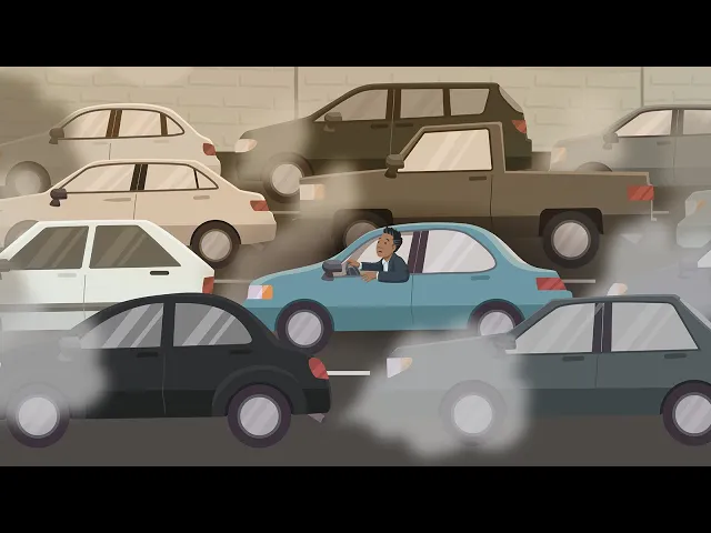
foreign executive editor of any JM evidence and this is stat [Music] uh traffic you're tired of spending so much time sitting in the car and spewing all that climate change inducing CO2 into the atmosphere you decide it's time for a change no more driving from now on you'll either take public transportation or bike to work but which is faster to answer this question you decide to conduct your own single commuter randomized control trial your trial design is straightforward each morning you'll wake up and flip a coin heads you take the train tails you get on
your bike just think about all the data you'll gather but before you start your trial you'll need to specify a plan for analyzing your data let's consider two possible approaches frequentest and Bayesian you first consider the more common frequentest approach When comparing two groups like cycling days versus train riding days the frequentest approach assumes that there is a fixed but unknown difference between them when it comes to the outcome of interest in this case the time to get to work you don't know what this true difference is but if you collect data for a period
of time you'll have a sample you can use to estimate it the difference between cycling versus train riding in your sample is an estimate of the true difference as usual the larger the expected difference the smaller the sample size that will be needed to detect it each time you do such a trial you'll get a different estimate if you do the trial many many times you could plot out the distribution of your estimates this is the heart of the frequentest approach estimates have a random distribution but the true difference is fixed the difference you find
in your data is your estimate of the true difference the population parameter but your data also tell you something about the distribution of estimates you would likely get if you did repeat the trial many times you can determine a confidence interval the confidence interval is defined by an upper and lower bound and a confidence level typically 95 percent and indicates that if you repeated your trial many times the true difference would be in that interval 95 of the time remember the interval is based on the likely distribution of samples for any single sample you may
or may not have actually captured the true difference you can however use your data to make some inferences you can ask How likely is it that someone would get these data if there were no difference in the means between the groups this Assumption of no difference is called a null hypothesis you could calculate the likelihood of finding the difference you observed or an even larger one if the null hypothesis were true if this probability or P value is less than 0.05 the frequentest approach rejects the null hypothesis declaring that the data you observed would have
been very unlikely if there were truly no difference but what if there is no single true difference after all lots of things can change day to day sometimes there are delays on the train some warnings you might have bike trouble to account for the possibility that there isn't a single fixed value and that there's actually a distribution of the effect size you turn to a Bayesian approach the fundamental difference between frequentist and Bayesian approaches is that the frequentest approach treats the true differences fixed and the data is a random variable while the Bayesian approach treats
the true differences a random variable and the data is fixed since the true difference is a random variable it will have a distribution in the Bayesian approach you determine that distribution which is referred to as the posterior distribution to do this you will need more than just your data you also use any prior information you have on what the distribution looks like for example maybe you've ridden the route to work before and you have a sense of the time it took from your smartwatch or if you're aware of electrical fires delaying trains recently you might
think that the distribution should be weighted towards the train taking much longer you use this knowledge to form a distribution you expect called a prior distribution your data will then allow you to alter your prior distribution into one more consistent with the measured data your posterior distribution which is the probability distribution of the effect size given the observed data and the prior distribution you can use your posterior distribution to calculate the probability of Any Given effect size the distribution of the effect size is often described by specifying the interval that contains 95 percent of the
distribution the so-called 95 percent credible interval this is tough stuff so let's work through your example you decide to conduct a Bayesian single commuter RCT you've heard that the electrical fires on the train issue has been fixed and based on your past rides you think that cycling takes about as long as a train ride with no slowdowns so you use a neutral prior in other words your prior distribution says it's equally likely that cycling or riding the train is faster after compiling a Year's worth of data you calculate that there's a 95 percent probability that
biking is faster than taking the train and that the 95 credible interval runs from biking being one minute faster to 10 minutes faster with the frequentest approach the p-value and confidence interval would have allowed you to reject the null hypothesis because biking was indeed faster plus or minus some number of minutes but with the Bayesian approach and further analysis of the posterior probability distribution you're able to see that there's only a 50 chance that biking is more than two minutes faster so it turns out that even if biking is faster it's not likely Faster by
much so taking the train is still a reliable option when you need it congratulations on conducting your first Bayesian analysis happy commuting just leave the car at home