Round Robin Scheduling (Turnaround Time & Waiting Time)

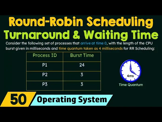
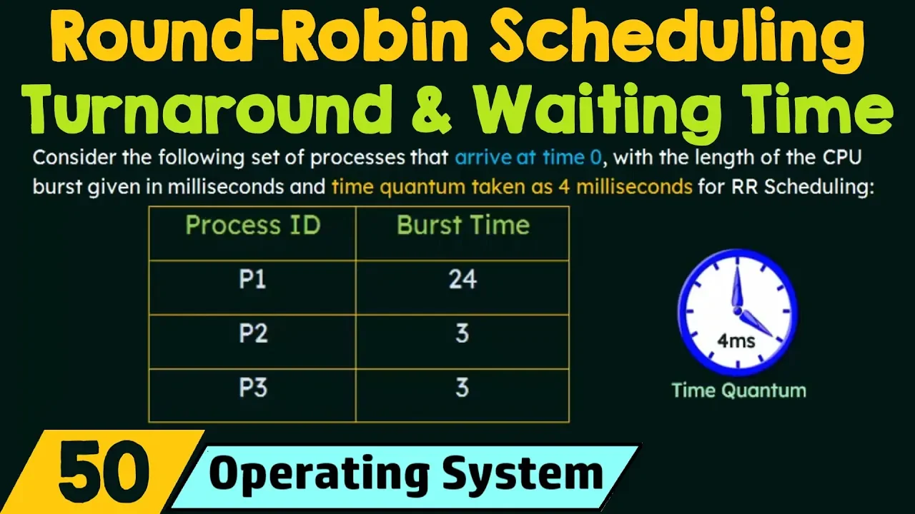
in the previous lecture we have studied about round-robin scheduling and we have seen how it works so in this lecture we will be seeing how we can calculate the turnaround time and waiting time for a round-robin scheduling so we will be taking an example of a CPU that follows a round-robin scheduling and we will see how we can calculate the turnaround time and waiting times for the set of processors in that so here consider the following set of processes that arrive at time 0 with the length of the CPU burst given in milliseconds and time

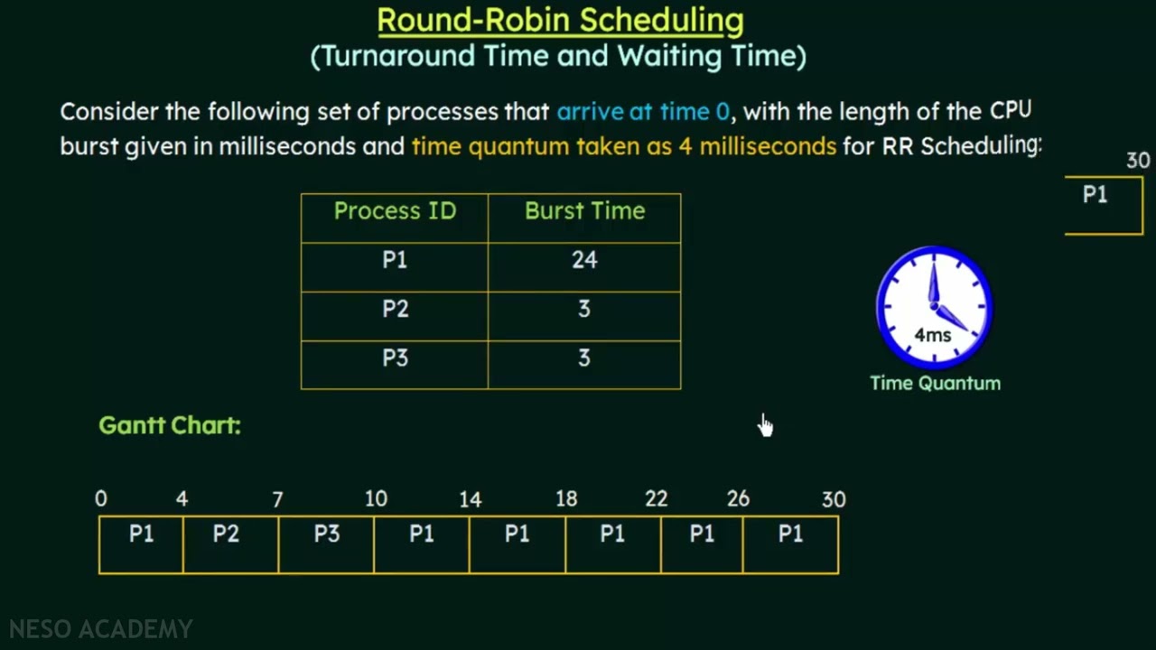
quantum taken as 4 milliseconds for round-robin scheduling so here we are given a set of 3 processes with process IDs P 1 2 P 3 and there both times are given in milliseconds so P 1 has a burst time of 24 milliseconds P 2 of 3 milliseconds and P 3 or so 3 milliseconds and we assume that all these processes arrive at time 0 so the arrival times for processes P 1 2 P 3 is time 0 and the time quantum is taken as 4 milliseconds and it follows a round-robin scheduling so if you remember

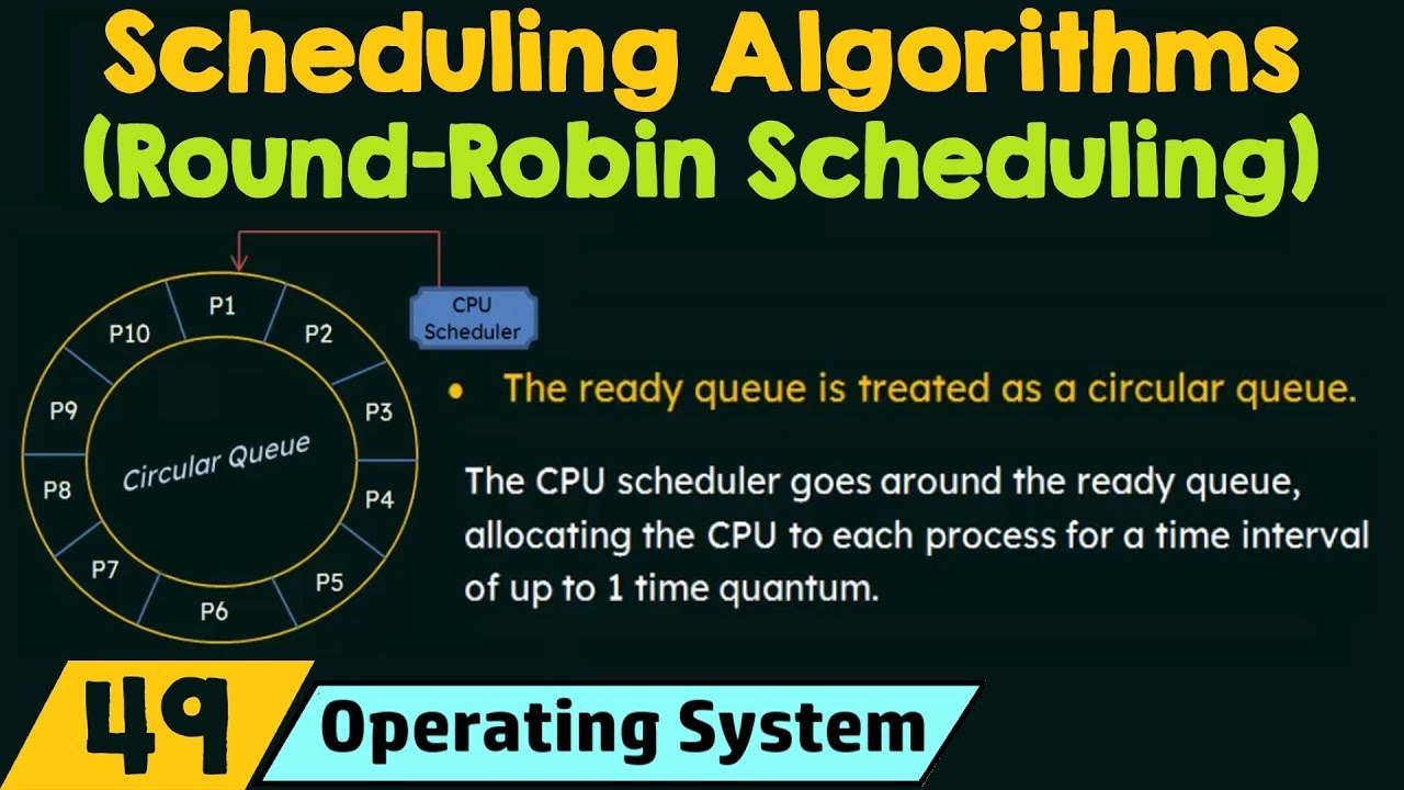
what I taught in the previous lecture about round-robin scheduling we have seen how it works so there we saw that in round-robin scheduling we have a particular time quantum which is a particular amount of time that will be assigned to each processes for their execution so a particular process will be allowed to use a cpu for a particular quantum of time that we define and once that time period expires the process will be preempted and the next process in queue will be given the CPU for its execution we should also be allowed to use the

CPU for a particular time quantum and then it will be preempted and the next process will be given the CPU and so on so that is our round-robin scheduling works which we have explained in detail in the previous lecture so here in this example that we are taking the time quantum is 4 milliseconds that means each of the processes will be allowed to execute for 4 milliseconds and after that the CPU will be given to the next process in the queue which will also be allowed to use a CPU for 4 milliseconds and then that

will be preempted and so on so here the time quantum is 4 milliseconds so here we will be seeing how we can calculate the on time and waiting time for this set of processes so the first step in calculating this turnaround time and waiting time for any scheduling algorithm that we have is to first form the Gantt chart so we have to form the Gantt chart for the set of processes and after that we would be proceeding to calculate the turnaround time and waiting time so let us see how we can form the Gantt chart

for this so here I have shown how the Gantt chart will be formed and I'll be explaining this but before that keep in mind that here we are following round-robin scheduling and we are to consider the time quantum which we have and the time quantum is four milliseconds so four milliseconds is our time quantum keep this in mind so we know that all this processes p1 to p3 they arrive at time zero so they are waiting in this order p1 p2 p3 in the ready queue so p1 is the first one that we have and

p1 will get the CPU at the zero at millisecond so when p1 gets the cpu it has to execute for how long the burst time of p1 is 24 milliseconds but will it be allowed to execute for 24 milliseconds no because this is round-robin scheduling and we have a time quantum and it will be allowed to execute only for that particular period of time which is 4 milliseconds in this case so p1 will be executed for 4 milliseconds so from 0 to 4 milliseconds p1 execute and after that what will happen P 1 will be

preempted and the cpu will be given to the next process in the cube so which is the next process in the queue it is p2 and what is the burst time of p2 p2 is first time is 3 milliseconds so at the fourth millisecond p1 is preempted and p2 now gets the CPU now p2 also will be allowed to execute for 4 milliseconds which is the time quantum but we see that the burst time of p2 is only 3 milliseconds it is less than the time quantum so it will execute only for 3 milliseconds so

p2 executes for 3 milliseconds which is from 4 to 7 so at 7 milliseconds p2 will voluntarily release the CPU because it's burst time was only 3 milliseconds which is less than the time quantum so we don't have to pre and p2 but it will voluntarily by itself or release the CPU now at 7 milliseconds CPU will have to be assigned to the next process in the cube so which is the next process it is P 3 so P 3 gets the CPU at 7 milliseconds and how long it has to execute it has to

execute for 3 milliseconds so again we see that the burst time of P 3 also is less than the time quantum of 4 milliseconds so P 3 executes from 7 to 10 that is for 3 milliseconds and it will also voluntarily release the CPU by itself so at the tenth millisecond P 3 finishes its execution and if we look here there are no more processes here but what actually happened was that P 1 it only executed for 4 milliseconds that is for the time quantum but it still has to execute for 20 more milliseconds because

only 4 milliseconds was executed so if we subtract 4 from this 24 which is the burst time of P 1 we see that it has a remaining burst time of 20 milliseconds so it has to execute for 20 milliseconds more so what happened was that when P 1 was allowed to execute for 4 milliseconds here and at the time it was preempted P 1 was taken and put at the end of the queue so the queue looked something like P 2 P 3 and P 1 because P 1 is again coming at the end of

the queue so when P 3 completes his execution there is P 1 still waiting at the end of the queue so P 1 will have to be given the CPU so P 1 will get the CPU when P 3 releases it and it will be executed for how long we see that it will be executed only for the time quantum of 4 milliseconds so P 1 execute from 10 to 14 milliseconds now did P 1 complete its execution now no P 1 has not completed its execution let's see how much did P 1 execute P

1 executed for 4 milliseconds here then here P 1 executed for another 4 milliseconds which is 4 plus 4 8 milliseconds so P 1 still has a remaining of 16 milliseconds to execute so P 1 is still there in the queue so at the 14 millisecond P 1 will again be preempted because that is the way round robin scheduling works after the time quantum of 4 milliseconds the currently executing process has to be preempted but we see that there are no other process other be one in the queue so it will be p1 being preempted

and p1 itself being given the cpu in this case so at the 14 millisecond p1 gets preempted and again p1 will be given the cpu because there are no other processes waiting in queue other than p1 so p1 will again execute for 4 milliseconds which is 14 plus 4 up to 18 milliseconds now did it complete no it did not complete now p1 how much did it execute here we see 4 here another 4 here another 4 so a total of 12 milliseconds were executed and there is a remaining of 12 milliseconds that p1 has

to execute because the total bus time is 24 milliseconds so again p1 gets preempted here and again p1 itself gets the cpu here so from 18 to 22 that is for 4 milliseconds it executes again and then here again p1 gets preempted and again p1 gets to CPU and it executes for 4 milliseconds and again the same thing happens here so from 26 to 30 milliseconds p1 will do its final execution so if you see the burst time of p1 is 24 milliseconds and it executed here for 4 milliseconds plus 4 here 8 and plus

4 here again that gives us 12 and if you plus 4 here again that gives us 16 then if you plus 4 here again that gives us 20 and if you plus 4 here again that gives us 24 milliseconds so then is how p1 completes his execution and the 30th millisecond so here we see that each process is allowed to execute only for the time quantum of 4 milliseconds so at the end even though it was only p1 that was waiting in the queue p1 will execute only for its 4 milliseconds then it will be

preempted but since it was the only process in q3 1 itself will be given the cpu and it was executing again and again so that is what happens in a round-robin scheduling so if there are more processes you can do the same thing and remember that a process that is preempted will be always put at the end of the queue so all the process will be executed and the process that is preempted will always be put at the end of the queue so keep that in mind and then you will be able to easily form

the shot for this all right now we have formed a Gantt chart and now let's see how we can calculate the turnaround time and the waiting time for round robin scheduling so I've copied down the same table here which shows our process IDs and the burst time and the Gantt chart that we have formed just now so now let's see how we can calculate the turnaround times and waiting times so for this round robin scheduling there are two methods in which we can calculate the waiting times so let's see what are those two methods so

the first method is using the formula that we have used for even the other scheduling algorithms that is turnaround time is equal to the completion time minus the arrival time and then the waiting time will be the turnaround time - the burst time so from the completion time that means when the process completely finishes execution from there if we subtract the arrival time we'll get the turnaround time and from the turnaround time that we just calculated now if we subtract the burst time then we will get the waiting tang so this method will be useful

when we you have to calculate both turnaround times and waiting times for a set of processes so let's see how we can calculate the turnaround and waiting times using this formula for this set of three processes so here I have a table where I have shown the process with process IDs P 1 2 P 3 and here we have the completion times of each of this processes so to see the completion times we can just look at the Gantt chart and find it out if you see for process p1 when did it completely finish its

execution so we see that p1 completely finished his execution over here at the 30th millisecond so that is the last occurrence of p1 in the Gantt chart so that will be the completion time that is 30 milliseconds now for p2 when did it last occur it was here and what was the time it completed 7 milliseconds so 7 is the completion time for p2 and for p3 similarly it last occurred here and this is where it completed its execution so 10 milliseconds is the completion time of p3 now let's calculate the turnaround time so the

turnaround time for P 1 will be the completion time - the arrival time so what is the completion time it is 30 milliseconds now what is your arrival time in the question it was already given that all these processes arrived at time 0 so the all arrived at zero milliseconds so the arrival times are zero for all the processes that we have here so the turnaround time of process p1 will be 30 that is the completion time minus zero which is 30 milliseconds now similarly for p2 what will be the turnaround time it is the

completion time 7 minus zero which is 7 milliseconds and similarly for p3 also the turnaround time will be the completion time 10 minus the arrival time 0 that is 10 milliseconds all right so we can easily calculate the turnaround times like this so in this question 2 arrival times were all 0 so in some other problems you may have different arrival times so if you are having different arrival times then use the arrival times as given in the problem all right now we can calculate the waiting time so the waiting time is the turnaround time

- that was same so turnaround times we just calculated here and the burst time is what is given in this table so for process p1 the waiting time will be the turnaround time 30 minus the arrival time 24 which is 30 minus 24 6 milliseconds and for p2 the waiting time will be the turnaround times 7 minus the burst time of 3 which gives us 7 minus 3 4 milliseconds and finally for p3 the waiting time is turnaround time 10 minus the burst time of 3 so that gives us 10 minus 3 that is 7

milliseconds so here we have calculated the waiting times as well so you can use this method when you have to calculate both turnaround times and waiting times so you can calculate turnaround time like this and once you have calculated turnaround time you can easily calculate the waiting time so now we'll go to the second method and in this method we will calculate only the waiting times so this method will be useful if you have to calculate only the waiting time and you don't have to bother about the turnaround time so here the formula that we

have is waiting time equals last start time minus the arrival time - pre emption into time quantum so this formula may look long but it is very easy let's explain it so last start time means the last time that the process started its execution so for example for p1 we see that p1 started its execution here at 0 milliseconds but was this the last octane no because p1 again started execution here at 10 milliseconds and here again at 14 milliseconds it started then again at 18 also it started then 20 to 26 also it started

so we see that the last start time of p1 was 26 milliseconds this is the last time it started so when it started at this 26 milliseconds it completed his execution at 38 millisecond and after that it did not start again so 26 is the last start time for p1 and from that we have to subtract the arrival time so for this example the arrival times are zero for all the processes and then from there we have to subtract the preemption into time quantum so preemption means the number of times the process got preempted so

how many times did p1 get preempted let's see so p1 got the cpu here and it was preempted and the CP was given to p2 then again here we see p1 got the cpu and it was preempted and was again given to p1 so from here also he was again preempted and from here also it was preempted and from here also it was preempted now when it got the cpu here for the last time at this point of time it completed its execution so there is no preemption happening here so how many times did p1

get preempted altogether 1 2 3 4 5 so p1 got preempted 5 times so similarly you can check for other processes so preemption so here the preemption value is 5 the number of time the process got preempted so for p1 it is 5 into the time quantum so with that you have to multiply the time quantum so our time quantum was 4 milliseconds in this example so 5 into 4 you have to multiply that so when you apply this whole formula you will get the waiting time for a particular process so let's see how we

can do this so for process P 1 what is the last start time the last start time is 26 milliseconds as I already explained this is the last time it started so look at the Gantt chart and look for the last occurrence of that particular process and see what was the start time so that is the last hard time 26 minus your arrival time so we know that the arrival times are zero milliseconds for the set of processes so it is zero then from there we have to subtract preemption into time quantum so how many

times did p1 get preempted I just showed you that it got preempted five times so five into the time quantum which is four milliseconds so into four so what is the value that will get here twenty six minus zero minus 5 into 4 so if you multiply 5 into 4 we get 25 for 20 so 26 minus 20 is 6 milliseconds so that is a waiting time for p1 so if you see here here also we got the same thing 6 milliseconds for p1 so similarly let's calculate for p2 so for p2 what is the

last start time the last start time for p2 where is it it is here so if you see in the Gantt chart p2 occurred only one time so this is the first and last start time for P 2 so 4 is the last start time for p2 and then the arrival time is 0 and in preemption so how many times it did P to get preempted we see that p2 was never preempted p2 gone the CPU once and it completed this execution at that time itself so there is no preemption for p2 so the preemption

is zero so x the time quantum which is forced milliseconds so there is 0 into 4 so 4 minus 0 minus 0 into 4 gives us 4 milliseconds so finally for p3 we see that the last start time of p3 is 7 milliseconds so p3 also got the CPU just once and it completed its execution that time itself so this is the first and last our time so 7 is the last start time for p3 and then the arrival time as we know is 0 and the preemption so we see that p3 also was never

preempted so it is zero into the time quantum which is 4 milliseconds so 7 - 0 - 0 into 4 so that will give us 7 milliseconds so if you compare here and here we see that in both the methods we are getting the same answer so this first method can be used when you have to calculate both turnaround time and waiting times and the second method can be used if you only want to calculate the waiting times so that is how you calculate the turnaround time and waiting time now let's see if we can

find out the average turnaround times and waiting times for these two methods for this set of processes so here we calculate raised on wrong time and waiting times average turnaround time for this set of processes where 30 plus 7 plus 10 divided by the number of processes that is 3 that gives us 47 by 3 that is fifteen point six six milliseconds and the average waiting time is six plus four plus seven divided by the number of processes three that gives us 17 divided by three that is five point six six milliseconds so similarly for

the second method also is the same thing average waiting time 6 plus four plus 7 divided by three that gives us five point six is milliseconds so in most of the problems you may be asked to calculate the average turnaround time and the average waiting times so if you have to calculate both of them you can use the first method or if you have to calculate only the waiting time you can use the second method so there is how you calculate the turnaround time and waiting time for round-robin scheduling so form the Gantt chart carefully

and apply these formulas and you can easily calculate it and also we see that in this round-robin scheduling the waiting times may be a little longer as compared to other algorithms because this algorithm is mainly used for time sharing systems and we have to carefully define the time quantum because if the time quantum is too long this round-robin scheduling will become like a first-come first serve scheduling and it is not useful and if the time quantum is too short then there will be two mini context switches happening so we have to strike a balance between

the two in order to maintain the efficiency of this algorithm so I hope this was clear to you thank you for watching and see you in the next one [Applause] you [Music]