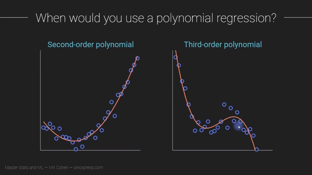
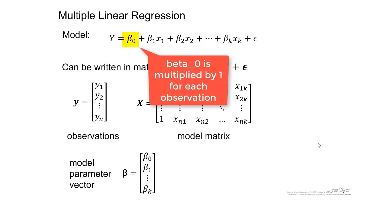
[Music] foreign [Music] and welcome back today we're going to continue our exploration of regression analysis and extend the type of model that we're generally working with which is typically a linear model to start and increase that order from a degree 1 model up to a degree in polynomial regression model so let's first off start off by going over the basics Associated to linear regression and some of the things that we can sort of look at to determine whether a linear regression model is actually appropriate so let's assume we have this set of bivariate data plotted here in Gray obviously it appears to be increasing you don't see any periodic Behavior it doesn't look like an x squared curve or anything fancy so one would generally say that this is appropriate for a linear regression model and of course you can assess for example normality Hamas elasticity Independence and linearity of the means if you really want to go that route but probably one of the fastest ways you can do to analyze the appropriateness is to look at the standardized residuals or just the residual plot for this particular model so if we look at the residuals Associated to our particular X values with the X values in the horizontal and the residuals of whichever predictor you want to analyze X1 and X2 down to XP then if you look at the residuals for this model then they should appear to be randomly scattered for example from typically minus three to three especially if you're looking for example the standardized residuals so if you try to fit a line of best fit for example to the residual plot you definitely should get a line that's practically equal to the x-axis right so therefore you should not see any correlation between these data points in particular the r squared value definitely should be approximately equal to zero for the standardized residual plot but if we take a look at for example a data set that definitely should not follow a linear data set or a linear model for example let's assume we have something that looks like that then obviously fitting a line is not going to be appropriate and you probably want to fit for example a quadratic or a cubic or some other fancy model to this data for example we may say that for example a quadratic model appears to be the best fit for this data or possibly even a cubic model to fit that particular data set so for example this blue curve could be for example Y is equal to Beta 0 plus beta 1X and this pink model could be the quadratic extension of that model which would be for example Y is equal to Alpha zero plus Alpha One X Plus Alpha 2 x squared and the only reason I'm using Alpha instead of beta is because these coefficients beta0 and beta 1 are usually not going to be the same as for example The Intercept in the first order term for the associated quadratic model so I just want to avoid any confusion that could result between these two very different models so let's start off with the very basic scenario of polynomial regression where we only have one predictor and one response so for example you want to see if there is a relationship between for example age and happiness and that relationship could either be linear quadratic cubic cortic but you believe that it is a polynomial Trend um between this predictor variable and this response variable so let's assume that our predictor variable is going to be represented for example by X and let's assume that our response variable is again y so our general polynomial regression model is going to be of the following form beta0 plus beta 1X Plus beta 2x squared that's going to be our quadratic model and then beta 3x cubed that's going to be our cubic model and we can continue this all the way out to for example beta P which would be a plus sign beta P times x to the power of p plus Epsilon where obviously P should be a natural number so that's our arbitrary simple polynomial regression model and um obviously we can write this as a linear regression model by simply redefining what our coefficients are because obviously X is just a variable so we can actually just call that X1 x squared is actually just another variable that happens to depend on X1 so we can actually just call that X2 we can call X cubed X3 and extend this all the way down to XP so we're going to have an equivalent representation of this model in particular Y is equal to Beta 0 plus beta 1x1 plus beta 2x2 plus beta 3x3 all the way down to Beta p x p plus Epsilon and notice that these coefficients are the same I've just redefined these uh predictor variables X1 down to XP into the integer positive integer powers of X right here x k is defined to be equal to x to the power of K and obviously K is a natural number right and we already know how to solve this particular model because we can vectorize this in Matrix form and write this as for example Y is equal to X beta plus Epsilon where X is an M by P plus 1 Matrix beta is a p plus one by one vector Epsilon is an M by 1 vector and Y is our n by one vector of response variables and we already know that for example an unbiased estimator for beta would be equal to Beta hat which can be found by X transpose X inverse times x transpose y as we've already proven for the multiple linear regression case okay so let's see if we can figure out how to build this particular data Matrix or design Matrix X so obviously our sample is going to be a bivariate sample because we just have an x value and a y value so our sets is going to be of the form X comma Y where obviously K is going to range from 1 to down to n and that should be x k and y k so if we just have technically one predictor then technically we just should have for example column of ones and a column of X ones inner design Matrix X so if we start by writing that out just to see what that would look like that means that our design Matrix X is going to be equal to 1 1 all the way down to one and then X1 X2 all the way down to for example x n and then it's going to come our X2 predictor variable values which are just going to be the squares of the linear terms so this is going to be for example X1 squared X2 squared all the way down to xn squared and obviously this is going to extend all the way down to X1 to the power of P X2 to the power of P all the way down to X N to the power of P um for our design Matrix X which obviously still is an N row by P plus 1 Matrix now this Matrix actually has a special form because it's just powers of that particular vector in particular that Vector to the power of zero power one power two all the way down to the power of p and this actually has a special name this is called a van dermond Matrix which of course has some linear algebra Theory Associated behind it now the first thing that I want to discuss in terms of some theoretical aspects about the vandermon Matrix that you should know is the determinant because we know that the determinant of a square Matrix being equal to zero implies that there is some dependence between the rows and or Columns of that particular Matrix so this theorem is as follows let's assume that a is a vandermond Matrix and when I say a vandermon matrix that means I have for example a column to the power of zero comma to the power of one a column to the power of two all the way out to for example com x to the power of n minus one right so let's assume that that is an M by n and hence has a determinant at least the classically defined and determinant then the determinants of this Matrix a is going to be equal to the product as J ranges from 1 to m of x k minus x j all right and that should be J less than or equal to K less than or equal to n all right so that's the general representation of this determinant but let's actually work through an example just to make sure we understand how it works so let's take a baby three by three Matrix for example let's consider the vector 3 4 5 raised to the power of 0 that's going to be one and raised to the power of two that's going to be 9 16 and 25. obviously our values are going to be X1 is equal to three x two is equal to 4 and X3 is equal to 5. so via this relationship for the determinant of this random Matrix you could either just find this via the classical expansion by sub matrices that would work perfectly fine it's the small Matrix it shouldn't be too difficult but this is going to be equal to so we're going to do 4 minus 3.
and then 5 minus 3 multiplied together and then we're going to shift up to the next element which is going to be 5 minus 4. so that's going to be equal to 1 times 2 times 1 which is going to be equal to 2 so that's going to be the determinant of this Associated veiner mind Matrix so when is this determinant equal to zero so the determinant of a van or my Matrix is equal to zero if and only if x j is equal to x k because that's these differences right 4 at least one pair of indices J K right for example if any of these numbers in this particular column repeat then that entire row is going to be the same and obviously that is a dependent row and or column and hence the determinant will be equal to zero let's assume that you collect this small but sufficient by very data set with Five Points 0. 1 3.
5 is the first point 0. 5 4. 8 as the second point and so on if you were to plot this graph although small set of points on a Cartesian graph you may assume that the data set appears to be quadratically related or possibly even cubicle cubically related or what have you so one could ask okay let's just try a bunch of models for example a simple linear a simple quadratic a simple cubic and just see which one is best so the first thing that we obviously would have to do is create a response Vector y so Y is going to be equal to our responses so 3.
5 4. 8 5. 5 6.
1 and 3. 7 our predictor values X is going to be equal to 0. 1 0.
5 0. 7 1. 1 and 1.
7 and obviously that's going to be defined as X1 for our first order linear term vector and then obviously x k is going to be equal to each of those values 0. 1 0. 5 0.
7 1. 1 and 1. 7 each raised to the power of K and I'm actually just going to write that as X 1.
to the power of K since we're just exponentiating each of those terms element wise right and if you're working in the r programming language defining that would work sufficiently so once you have that and you can solve multiple linear regression models now we can just try to fit a bunch of things together so for example let's assume we're interested in a first order linear model in particular one the form Y is equal to beta0 plus beta 1X Plus Epsilon one can find that the predictor model y hat is going to be equal to approximately 4. 01 plus 1. 35 times x so in terms of determining whether this model is appropriate or not there's two common measures that some people usually result to the first is the p-value because that's looking to see if we should reject whether or not the coefficient of beta 1 is close enough to zero to imply that the model's not appropriate so one can find that the p-value is approximately equal to 0.
0993 which is relatively small one could argue and if you look at the r squared adjusted value you can find that's approximately equal to five three three five which is not exactly close to one but some people may argue that it is right but generally speaking the p-value could be a lot smaller and the r squared value could be a lot larger so generally speaking one could say that these metrics are not so great so if that is the case maybe you would consider increasing the order of our model for example to a degree 2. so a degree 2 model would be equal to what so that would be for example Y is equal to Beta 0 plus beta 1X Plus beta 2 x squared plus Epsilon and obviously these betas are not the same betas because they're corresponding to two different models now before we start analyzing the model you have to Define how good is good in terms of the metrics for what you're aiming for because one will find that as you increase the number of predictors just like a multiple linear regression the SSE will always converge to zero right in particular we're going to have an overfitting issue right so for example let's define our ideal values for example we can say that Alpha as our 0. 05 so once we get a p-value below that then everything is wonderful and let's assume that an ideal r squared adjusted value would be let's say 0.
85 right so let's assume we Define these as good so once we have one or both of these metrics satisfied then we could say that that is the order model that we should reach so if we fit this model via multiple linear regression we can find that the predicted model y hat is going to be equal to approximately 2. 98 plus 4. 90 x minus 1.
93 x squared and then we can get our model assessment parameters in particular our p-value when combined is approximately equal to 0. 0073 and the associated r squared adjusted value is approximately 0. 9853 notice that both of our ideal criteria are met therefore we should be very satisfied when we see that therefore you should stop increasing the order and say that M2 a beer appears to be a better fit for our model but let's just actually go ahead and calculate what M3 will generate so that's going to be our degree 3 Model one can actually find that the p-value is going to be approximately 0.
0654 and the r squared adjust a value is approximately 0. 9894 obviously the r squared to just a value does increase closer to one the p-value does not converge to zero uniformly but as you make the number of predictors go to Infinity eventually the p-value will be monotonically decreasing to zero but I won't get into the proof of that at least for right now right but you should not be surprised that the r squared value is decrease or increasing every time we add a predictor because that's one of the properties of the r squared and r squared adjusted metrics so there's obviously two issues that we definitely need to be paying very close attention to the first thing that we need to avoid obviously is overfitting so overfitting is the sense when we're forcing our SSE to converge to Zero by increasing the number of predictors in our multiple linear regression model but generally speaking you should be able to prevent overfitting by implementing some sort of self-control by pre-defining your Alpha value or predefining an ideal r squared adjusted value or some other metric that you have in front of you the second issue that we have is what is referred to as structural multi-co-linearity some people just call it structure co-linearity or just multicolinearity and what that is is when we introduce for example a predictor and that predictor raised to a power obviously these two variables are dependent by Design and we already know that predictors on the mount on their own is a very bad thing right so we're introducing correlated random variables in our data and that of course is going to lead to some very bad issues for example let's look at a couple metrics that we already should be familiar with analyzing in terms of diminished dependence and multicollinearity from the multiple linear regression perspective so let's assume that P corresponds to the number of predictors which at least for polynomial regression is the order of our simple polynomial regression model and let's consider one two and three for the same exact data set that we've actually been working with for the past couple of statements so we've already calculated our models one two and three let's consider for example the condition number for The Matrix X which is just the quotient of the maximum and minimum singular values of that Matrix and let's also do the square root of the determinant of X transpose X which can be viewed as the pseudo determinant of the Matrix X since it's not technically Square so one combined that the condition number for our models 1 2 and 3 is 3. 31 15.
2 and a number approximately equal to 100 and the square root of the associated determinant of the x t x matrices for each of these models one can find is 2. 73 1. 69 and 0.
37 as we can see we can see that the condition number is getting larger which is typically the case and the current in the determinant is getting smaller so we already know that when the condition number gets larger that means the Precision and stability of our model is getting worse and when the determinant is getting closer and closer to zero that means the Matrix is the Matrix in particular of x t x is getting closer and closer to a singular Matrix which means that the solution of our multiple linear regression equation you know the beta hat is equal to x t x inverse x t y is becoming more and more less reliable and eventually will not exist since the inverse will not exist so both of these are definitely a very bad thing so how are we going to go about fixing these issues that we have by Design created in our polynomial regression model one common method that is often used to reduce the structural multicollinearity issues of polynomial regression models is what is known as variable standardization which actually can be used for practically any regression model and will also be used in some later Advanced statistical techniques such as principal component analysis but what is variable standardization so the root of the word standardization in particular standardized should sound familiar and it definitely is going to be used here and that's the standardization of variables so what we're going to do is going to Define what is called a standardized predictor which is going to be represented by z k which is going to be the original predictor minus the mean of that predictor divided by the standard deviation of that predictor so here these are all constants and these are element-wise operations on this particular Vector x k therefore once you standardize each of your predictors X1 X2 down to XP then you have what is called the standardized polynomial regression model so the standardized polynomial regression model is going to be of the following form keep in mind we only have one predictor therefore you should only be standardizing one vector therefore our standardized polynomial regression model is going to be equal to Y is equal to beta0 plus beta 1 Z and then plus beta 2z squared so that's just a squared value of the Z standardized values and that's going to continue all the way up to Beta p z to the power of p plus Epsilon so that's our standardized regression model now let's look at the differences and similarities between the original model and the standardized regression model just to see how we can interpret and see the pros and cons of this original model so let's consider for example the quadratic model for the same data that we had before which keep in mind we had the model the quadratic model approximately 2. 98 plus 4. 90x minus 1.
92 minus 1. 92 x squared and one can find that the condition number for that model again is approximately 15. 2 and the p-value actually let's do the square root of the determinant of X TX that's approximately 1.
69 the p-value for that model is approximately 0. 0073 and the r squared adjusted value is approximately 0. 9853 and also let's just mention one of the standard errors in particular the standard error beta0 since that's usually the largest one that's approximately equal to 0.
15 now let's look at the same metrics but for the standardized version of the quadratic model let's call that m z two so one can find that the coefficients of this model is going to be approximately equal to 5. 70 plus 1. 60 Z minus 0.
72 Z squared so for our metrics one can find that the K Matrix or the condition number for X were technically Z is going to be approximately equal to 2. 7 the square root of the determinant of x t x is going to be approximately equal to 7. 45 the p-value approximately 0.
0073 and the associated r squared adjust the value of approximately 0. 9853 so to compare notice the p-values and the r squared adjusted values are the same exact thing right so therefore it has the same model predictions and of course they have the same exact accuracy right but if you look at for example the condition number and the determinant which used to be large and small respectively now we have small and large condition and determinant respectively right so determinants gotten farther from zero our condition numbers got closer to one right so that means that the model has better precision and stability also another Advantage is that the coefficients for this model are all going to be in the same exact unit in particular they have no units right so that's a good Advantage especially for standardizing predictors for a general multiple linear regression model not necessarily a polynomial one right so if you look at for example the standard error for the beta hat zero term for the standardized model one can find that that is actually approximately equal to let me see what that is that's going to be approximately equal to 0. 08 so notice that the standard error Associated to 1 and usually all of your predictor coefficients are usually a lot smaller to work with and that of course ties in to the accuracy precision and also the stability and accuracy of your Associated regression model so in general every time you're working with a polynomial regression model you should always be standardizing your predictors to make your model a lot more precise and a lot more stable the last thing I want to discuss today is how to build what is called a multiple polynomial regression model if you have more than one predictor and you want to use a polynomial regression model on each of those predictors so let's assume as an example that we have three predictors let's call them X1 X2 and X3 and let's assume that we want to build a general quadratic polynomial regression model for these three predictors what would that model look like so let's assume that we have just one response variable Y and we're obviously going to have our beta 0 intercept but some people choose that to be zero but I highly do not recommend allowing your beta 0 to be zero even if you're standardizing your predictors for a variety of theoretical reasons so then we're going to look at for example the linear terms for a model so let's call them the following let's call it for example beta 1 1 x 1 plus beta 1 .
let's call it beta 1.