(upbeat music) - Hi everyone. Welcome back to coding with Qiskit. I'm your host Jin.
In this series we cover topics in quantum algorithms each week. So be sure to like and subscribe. Today we're gonna be talking about one of the most well-known ways a quantum computer can outperform a classical computer using the second most famous quantum algorithm, Grover's algorithm.
Before we get into that, let's talk about what a quantum algorithm is and what advantages they provide over classical algorithms. A quantum algorithm is a set of instructions that's run on a quantum computer that takes advantages of the quantum properties of superposition, entanglement and interference. A classical algorithm is run on your laptop at home, which uses binary logic.
So let's talk about the problem that we're gonna solve with Grover's algorithm into how a quantum computer would approach the problem versus a classical computer. Later on I'll walk you through how you can implement Grover's algorithm yourself in Qiskit So let's go ahead and open our Jupyter notebook so we can get this started. I'm going to open up my coding with Qiskit environment.
So conda activate coding with Qiskit. And this is where I have Qiskit installed. I'm gonna just open up a Jupyter notebook so we can get this started.
I'm gonna open up a new Python 3 notebook. Suppose we have an unsorted list of N elements, and we wanna locate a particular element of the list that we'll call the winner w so I'll just make my list here. (indistinct) I'm just filling it with random numbers.
So let's say from this list of numbers I wanna find where the number seven is in this list. How a classical computer would approach this problem would be to check each element of the list here and just see if that number is equal to my winner. And we can model this using what's called an oracle.
And all this means is that we have a black box at our disposal and we can call it and ask it, is this number the winner? Yes or no. So let me just define my oracle My input.
And the oracle knows that my winner is number seven. And it'll just tell me if I give it an element of the list if that element is the winner. So if my input is winner, response equals true else response equals false return response.
So now let's see how many times we have to call the oracle in order for us to find the actual winner. So for index and trial number and numerate my list. If the oracle if I give it my trial number, and if it's the winner then give me back this print statement winner found at index I and tell it to print my index.
Also oops. Also tell me how many times I had to call the oracle. And break.
Okay. So what this is telling me is I had to call the oracle 10 times and the winner was found at index nine of my list. And we can just quickly verify that.
Seven is the ninth index of my list. So we use 10 calls to the oracle. So we see for this list, it took us 10 calls to the oracle but we can also imagine a situation where I get lucky and my element is at the front of the list.
So we would use fewer calls to the oracle. So on average, the complexity of this problem requires us to call the oracle N/2 times on average. In the worst case, I would have to call the oracle N times if my element was at the very end of the list.
So we say that the complexity of this problem scales as order N in the classical case. Now the amazing thing about a quantum computer is that we can get away with only square root N calls to the Oracle by using Grover's algorithm. So let's get into how this algorithm works.
The oracle in the quantum case. I'm going to just model at this black box, oracle And it's given me a function that will flip the sign of the input if the input is the winner. So we can encode our inputs as the basis state of a quantum computer.
So remember for two qubits, we can represent four input states. 00 01 10 and 11 and let's suppose that our winner is the state 11. So if we feed our state 11 into our oracle, where we get back is minus 11 and this is the way oracle is gonna work.
It's gonna flip the sign of the input if the input is the winner. And the way we can change these states is through a unitary matrix which we can encode into a quantum circuit. So we want a circuit that flips the sign of the 11 state and conveniently we have a gate that does just that the controlled-Z gate.
In addition we'll need one more ingredient in order to do what's called amplitude amplification. And that ingredient is called the reflection operator. The combination of these two operators is known as Grover diffusion operator.
Let's see what this looks like in Qiskit now. So from Qiskit I will import everything. Import matplotlib.
pyplot as plt, so I can do on plotting and I'll import numpy as np, just so I can do some array stuff. Okay. So let me now define the oracle circuit.
So the oracle equals quantum circuit with two qubits. I'm just gonna deal with two qubits for now. I'm going to call this the oracle.
And like I said before there is a convenient gate that flips the sign of our winning state with the controlled-Z gate. And I'm gonna make the oracle into its own gate. Let's see what this looks like oracle.
draw That's my CZ gate which acts as my oracle. Let's quickly check now that our oracle is doing what I want it to do. So I can check this by preparing a superposition state of all of my qubits by applying a hadamard gate on each one of them.
And this way I can query each one of the input states simultaneously to the oracle. I'll call the state s for superposition. so to check that the oracle is doing the right thing I'm just gonna call the simulator backend the state vector simulator.
Okay. I'm gonna define my Grover's circuit, quantum circuit, two qubits, two classical registers, grover_circ. And I'm gonna add hadamard gates on both of my qubits 0 and 1.
This prepares my superposition state s. And then I'm going to add on my oracle. So I can query each one of my states at the same time.
And let's once again draw this so I know what it looks like. Okay good. So I am applying a hadamard on each one of my input qubits, This prepares all four superposition states and then I feed them into my oracle.
So let's execute this job on the simulator. Get back the result. Okay.
And let's get back the state vector, result. get_statevector. And I'm just gonna round these numbers off.
Okay good. So we prepare the superposition state and we get back to the same state, but with the 11 state flipped. So our job is done, right?
Not so fast. In quantum mechanics, we have to square the state factor in order to get back to probabilities of measuring that state. More precisely, we have to multiply each element of the state vector by its permission conjugate in order to get back the probability of measuring that basis state.
So the minus sign in the state vector will never actually show up in any measurement that we do at this point. We need one more ingredient to tie all of this together, the reflection operator. With the oracle and the reflection operators, we can do something called amplitude amplification.
With amplitude amplification, we can amplify the probabilities of the winning state w and we can reduce the probabilities of all the non-winning states. Let's talk about how the amplitude amplification works now. There's actually a really nice geometrical interpretation of how this works.
So let's think about our winning state w. And our superposition state s. And our winning state is represented as this vector (0,0,0,1).
And this is equal to the 11 state. The superposition state is represented as this vector (1,1,1,1). Where each one of our input states is equally likely and normalized by one half.
So we can think about these two states as vectors in space, which are almost orthogonal or almost at the right angle but not quite. And we can come up with a new state within the span of w and s. Which we'll call s prime, which is actually orthogonal to w.
So this will be defined as (1,1,1,0) and with the normalization factor. You can actually check that w and s prime are orthogonal to each other. So you'll notice that s prime is just the s state with a w component removed from it.
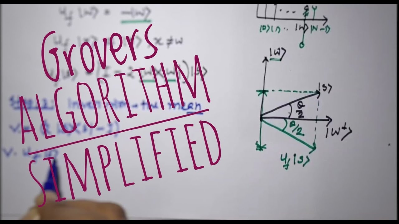
So let's draw what these vectors would look like in the space. Here I'm drawing my w vector. There's my winning state.
And like I said before, the s state is almost orthogonal to it, and we've constructed our s prime state, so that it is orthogonal to w. So this is a right angle here. So now when we apply the oracle operator to s.
So s goes into our oracle. The oracle flips the sign of the winning state. So what comes out is this vector (1,1,1,-1) and our normalization factor.
So now when we apply the oracle operator to s we flip the sign of the winning component. So geometrically this means that we reflect our original s about s prime. So we get a new vector that looks like this.
So our s has been reflected around s prime and goes here now. So now let's apply the reflection operator, which is defined as this. Minus the identity.
And what this is gonna do is reflect our new vector here about our original s vector. So what this looks like is something like this. So we started to here, we went here, and then we ended up here.
So you can see that the combination of these two operators actually brings us closer to our winning vector w here. In fact each time we apply these two operators, our quantum state moves closer to the winning vector. In our example of four elements, we'll see that we'll actually get the correct answer after one application of amplitude amplification.
For larger systems, the number of times we'll have to apply the amplitude amplification, will scale as square root N. Let's take a look at how this works in Qiskit. We have all the pieces in place except for the reflection operator now.
So one way of thinking about the reflection operator, is to apply a negative phase to every state orthogonal to our original s state. So let me start writing up this. (indistinct) So what we want to do is an operation that takes our superposition state back to the L zero state.
So we can do that by applying hadamards on every qubit and then apply a circuit that applies a negative phase only to the 00 state. So I'm going to add hadamards on all of my cubits to bring them back to your original 00 state from the s state. And then apply Z on both of my qubits and then a controlled Z.
And this is a circuit that will apply a negative phase only to 00 state. And then I'll transform it back with a hadamard on both qubits. I'll turn this into a gate.
And let's take a look at how the reflection operator looks. Okay good. Now let's put it all together.
So set my backend to a qasm simulator. Grover_circ equals quantum circuit, two qubits, two classical registers. I'm gonna prepare my superposition state, hadamards on both of my qubits.
I'll add my oracle and then I'll add my reflection operator. And then I'll add my measurements at the very end. Okay.
And then let's take a look at what the circuit looks like. Okay good. So we've prepared our superposition state, we have our oracle, and we have our reflection operator.
And what we wanna get back at the very end is the state 11. So let's execute this job, grover_circ, backend. .
. And I promise you that we'll get the 11 state back at the end. So I'm only gonna do one shot.
So let's get the results, result, and get the counts back. Okay great. So our result has given us back, the 11 state as promised.
So there you have it. We implemented Grover's algorithm and we only used one call to the oracle in order to find our winning state. Now remember classically, we would typically need to use of order N calls to the oracle if we have an N size list.
On the quantum case, by using amplitude amplification, we can get away with only using square root of N calls to the oracle. Why don't you try out this circuit on a real backend and let us know in the comments how it goes. Join us next week where we'll talk about quantum chemistry.
Thanks for tuning in and don't forget to like and subscribe. See you next time.