Hello everyone and welcome to another episode of coding adventures. Today I'd like to build a little tool for analyzing audio. So sound as we've very crudely simulated in the past is transmitted as waves of pressure.
And if we plot that pressure over time, we get some sort of signal such as this. We also implemented the discrete FIA transform which allows us to break a signal down into individual waves of constant frequency, phase, and amplitude. As you no doubt know, frequency is simply how many times a wave goes up and down in a single second, and it determines the pitch that we perceive.
For example, here's a 150 Hz wave, giving us a fairly low hum. And here is 350 Hz. Amplitude then affects how loud that sounds and it's measured as the maximum height of the wave from the baseline.
Finally, the phase is an angle which essentially acts to shift the wave sidewards. It's not super interesting in isolation, but if we have multiple frequencies added together, then their [music] phases can have a big effect on the shape. Anyway, breaking a signal down into individual waves, as I was saying, can be very helpful for understanding the sound better or making modifications to it, like eliminating an annoying high frequency, for instance, before adding the waves back together.
We played around with this sort of thing on much more complicated signals such as this voice recording here. Hello everyone. Like taking a look at the amplitudes of the various frequencies in there.
We tried reconstructing the signal with just a small subset of the most prominent ones in the code. That's done by running the input audio through our little FIA function, sorting the frequencies by highest amplitude first and then taking some specified number of them. Those are used to construct a new signal over here which is done by generating waves with the given frequencies, phases and amplitudes of goss and summing those all together.
So let's have a quick listen to how the audio sounds with just five frequencies involved. It's basically just a weird low pitched wobble. So here it is with 50, which is not all that much better.
And here's 500. This at last is at least discernible a speech. Although the quality is still quite horrendous, but I think the reason we needed so many frequencies to get here is that none of them in isolation really correspond to an actual sound being made in the speech.
Like to explain a bit better what I mean, let's consider a super simple signal that maybe starts out silent, then goes along at 8 hats for a brief moment before changing to 12 hats [music] for a bit and then falling silent again. So, we've made this out of just two frequencies, but they're switching on and off. In other words, their amplitudes change over time, which is not a concept that the FIA transform understands.
[music] So if we feed in the entire thing, it'll say the most prominent frequency in there is actually 10 herz followed by 12 Hz and then 11, then 8, and a whole bunch more. As we can see, even though our recording appeared very simple, the fact that it was changing over time means that the signal as a whole contains many, many more frequencies than we knowingly put into it. What we could imagine doing though is rather than feeding the entire recording to the FIA transform, we could chop it up into smaller segments to scrutinize separately.
That way, the function would ideally detect just the frequencies that were actually present at each moment in time instead of all these more abstract frequencies required to represent the entire thing at once. So going back to the voice recording, let's try slicing this into little segments now and run each of those through the FIA transform individually. This process is known as the shorttime FIA transform by the way.
And I've started out in the code with two little structures here. one for holding the frequency data for a single segment as well as keeping track of where in the signal that segment is situated and the other to simply hold all those segments along with the sample rate and number of samples in the original signal. To create all this, there's then this function over here that takes in a signal and the desired number of samples that each segment should contain.
So we can just run through the signal grabbing segments of that size to pass through the discrete for transform and store the frequency data from that in our segment structure. Those segments are then finally lumped together in our little result structure here for convenience. Now what I want to do to test this out quickly is just loop over each of the segments in the result we're getting back over here and reconstruct each portion of the original signal from the frequency data in those segments.
All right, I've run this here with 48,000 samples per segment to start with, which is actually all of the samples in this 1second clip. So, we unexitingly have just a single segment. Down at the bottom, by the way, we also have the amplitudes of all of the frequencies that make up the segment.
Then having a closer look at this info up here, we can see for instance the segment duration of a th00and milliseconds, which tells us that if we're trying to figure out when certain frequencies are present in our signal, well, we can't narrow down the time any more precisely than that. Finally, theory transform can analyze half as many frequencies as samples it's given. So 24,000 in this case, which is also the maximum frequency this recording can contain.
And so the frequency information we get back will be in 1 Hz intervals here. The reason for there being a maximum frequency, you might recall, is that we need at least two samples per cycle of a wave to capture how fast it's oscillating. And failing that, we run into aliasing issues, which is where a high frequency falsely appears as a low frequency in our recording.
Anyway, let's quickly listen to our reconstruction of the input signal here. Hello everyone. And that is identical to the original, but let's try chopping it up into maybe 10 segments now.
So that's 4,800 samples per segment, making each of them a 100 milliseconds long. So we have better time resolution now, but our sort of frequency resolution or whatever we want to call it has become correspondingly coarser. Let's have a listen to see if that impacts the quality at all.
Okay, it's quite subtle, but that does seem to be something slightly wrong there. Oh, this should be the number of samples per segment, not the number of samples in the entire thing. So, let's try it again with that fixed.
Hello everyone. And now our reconstruction is actually identical to the original again. Let's keep going though and try splitting it into a 100 segments now.
making each one just 10 milliseconds long but with a 100 hertz between each frequency. And listening to this, hello everyone. The reconstruction is still perfect.
However, what if we go all the way to the extreme with just one single sample per segment? In this case, we have the best possible time resolution matching the rate at which the audio was recorded, but we've traded away all of the frequency information. So if we browse through the segments here, we can see it's entirely made up of zero frequency waves just shifting up and down based on phase and amplitude.
The fo transform is essentially spitting back each sample we give to it just in a slightly different [music] format. And so if we play the sound, hello everyone. Unsurprisingly, it is identical to the original just like [music] the others.
So it seems no matter how we slice things, we can still reconstruct the original signal using the information from the FIA transform. But there's a fundamental trade-off in what we can learn from that information. At one extreme, we know precisely where we are in time while having no notion of which frequencies are present.
[music] And at the other, we have maximum precision about the frequencies, but have tragically lost our sense of time. So depending on our specific goals, we just have to strike some balance, I suppose, between these two extreme uncertainties such that we're able to learn a bit about what's happening and a bit about when it's happening, too. Anyway, just for fun, let me actually play the audio while we're manually scrubbing through these segments here, so we can get a sense for how they sound in isolation.
[music] [music] Hello everyone. Okay, I'm kind of curious now what this would sound like if we limit it to just the single most prominent frequency per segment. But I'm a bit sick of hearing hello everyone all the time.
So I've quickly downloaded a giant list of adjectives and nouns and written a tiny Python program to print out a random pair. So our new phrase is going to be punctual thunderstorm. All right, I've set it up in the code to take just the frequency with the highest amplitude when reconstructing the signal.
And I also added a duration multiplier so we can slow down each segment. This works the same way as that accident earlier with the Okay, I've set the duration multiplier to eight so we can hear the individual tones nicely. And let's give it a go.
[music] [music] All right, that sounds pretty beepy, but let's try it again at just three times regular duration. [music] And that's sounding a bit closer to speech now. So, let's try it finally at regular speed, which sounds surprisingly good, I think.
I love how these almost random seeming little beeps and boops simply played at the right speed suddenly resolve into recognizable words. I'm curious to quickly hear how these tones change if we introduce just a few more frequencies, like maybe five per segment. Now, [music] right away, we can hear a little added complexity from those extra frequencies, of course, some of which sound quite unpleasant.
But anyway, let's go back to the start and see how it sounds if we scrub through at roughly real time. Oh, punctual thunderstorm. >> And okay, those few extra frequencies have definitely increased the clarity quite a lot.
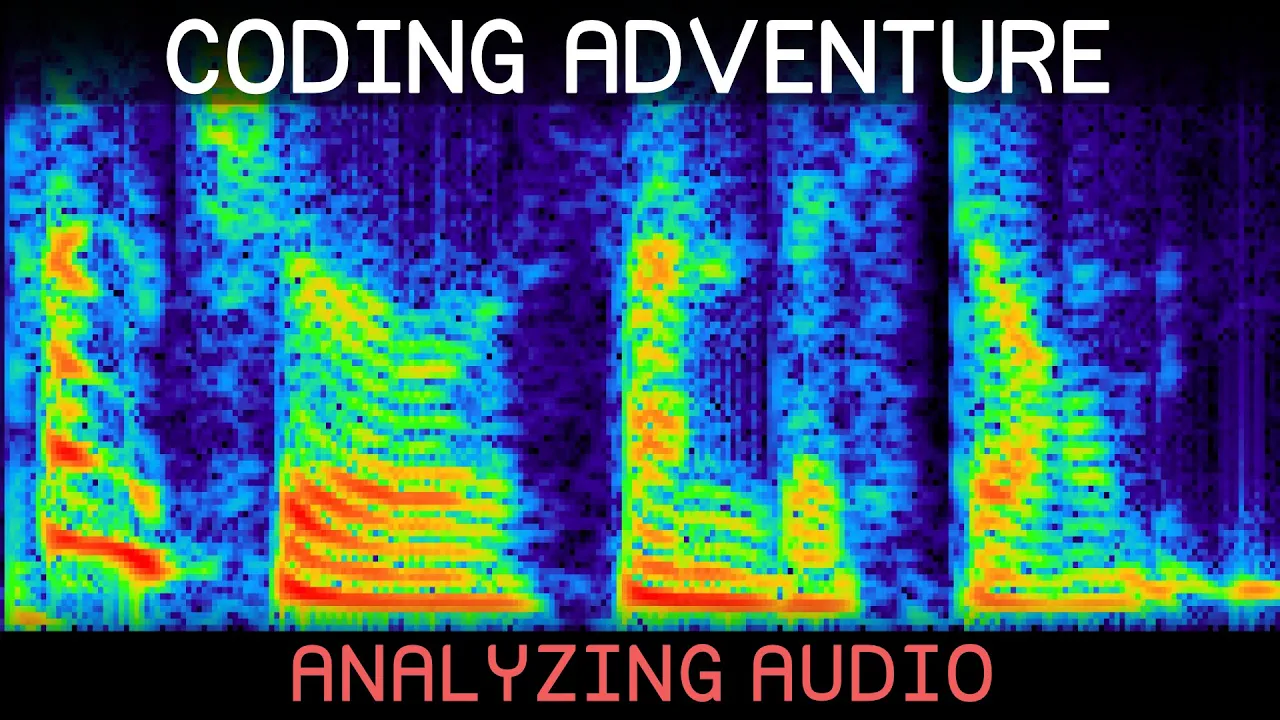
For comparison, here it is now with all of the frequencies involved. Punctual thunderstorm. Okay, enough messing about.
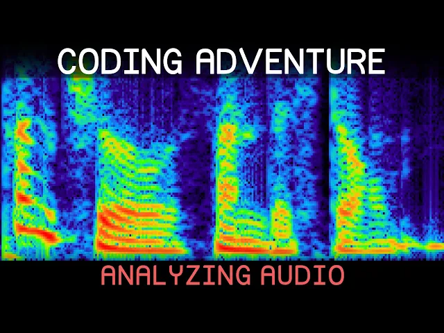
Let's actually visualize the data we're getting back from this short time for transform. Like we could have time running along one axis, frequency on the other, and use brightness to represent the amplitude of each spot on that plot. In other words, a spectrogram.
So, I've written this little function that takes in the data and just writes the amplitudes into the red channel of a 2D texture, which is then passed along to this shader over here. All this does right now is allow us to specify a range of frequencies we're interested in displaying, which then determines the vertical region of that texture that the shader will read the amplitudes from. And those will finally output as black for zero amplitude up to white for the maximum value.
All right. and running this now. Here's what we get for our punctual thunderstorm.
Okay, I think we need to do some tweaking. So, I'll adjust the maximum display frequency down to around 5,000 perhaps. We can see some interesting squiggles now, but overall it's looking more barren than I was expecting.
So, in the code, I've tried quickly converting the raw amplitudes into decibb instead, which should reflect a bit better how loud we actually perceive the sound to be. There are other factors that affect our perception of loudness like frequency and duration. But the important thing for now is just that a lot of the quieter details in our sound here have been brought to light.
Just out of preference though, I think I'll actually invert this so that loud sounds are displayed darker. All right, I think that's looking nice, but there is still something we should probably address, which is an effect we encountered last time called spectral leakage. Consider this five Hz signal over here for instance which has been sampled 64 times over a duration of 1 second.
And since this is a 1second recording, any integer frequency like we have here will appear periodic. Just meaning that when we get to the end, we can imagine on the next time step looping around and starting seamlessly again from the beginning. When we go and plug this into the FIA transform, we'll get back the amplitudes of all these frequencies here.
And as expected, the 5 Hz frequency has been detected. However, if the wave does not appear perfectly periodic, let's say it's 5. 5 Hz here instead.
In that case, the F transform is no longer able to pick out that precise frequency. Rather, the amplitudes around the true frequency are largest. But we can see it's been spread very broadly across the spectrum.
This leakage, as it's called, is obviously quite annoying if we're trying to analyze our signal. And so, one way to mitigate it is using a function like this one. The idea is just to scale our samples by this curve.
So the first sample would be scaled down to zero, then gradually they'd be allowed to reach their true amplitude in the middle before being smoothly scaled back down to zero at the end to match up with the beginning. And in that way, we're forcing the signal to be periodic. Okay, I've implemented this quickly over here, just simply looping over the given samples, figuring out how far along we are as a value between 0 and one, and using that to evaluate our smoothing function, which finally, of course, scales the current sample.
All this scaling is also going to scale down the amplitudes we get back from the FIA transform. But I think we can counter that side effect by just dividing those by the average value of the smoothing function which is 0. 5 for this particular one.
So let's return to our very leaky spectrum [music] over here and see how it changes when we apply all of this. And okay, we can see that the amplitudes are still spread out a little since this obviously isn't a pure single frequency anymore after our tampering. But we have managed to confine that spreading for the most part now to just a few frequencies.
I want to see quickly what happens as we increase the true input frequency here. [music] And it looks like the extent of the spreading is remaining very consistently focused around that true frequency. So this consistent behavior we have now should hopefully make our lives easier if we're trying to perform some sort of analysis.
Let's also test quickly how this behaves when we take just a subset of the samples like we're doing with our shorttime shenanigans. So fewer samples means less frequency resolution as we know. But the results still looking good.
And if we shift our window around to grab different parts of the signal, that is looking nice and steady too. For comparison, here's how it looks without the smoothing. Okay, returning to our spectrogram at last.
Applying that smoothing window here takes us to this, which doesn't look like a super dramatic difference, but I'm still glad we took the trouble. Now, there's one last little improvement I want to make to this for now, which is to take the segments we're chopping the signal into and add an option for overlapping them. The purpose being that we can then fit [music] more segments in without having to make them any smaller, which will give some extra visual smoothness along our time axis.
In the code, this just means an additional parameter called the hop size is now passed in alongside the segment size. And we'll simply increment the starting index of each segment by that hop size instead. So here's how it looks if we go down to a hop size of 1/2 the segment size for instance, which is certainly a bit less blocky.
We can also play around with the segment size itself, of course. Like we can see some of these frequencies here look kind of smooshed together at the current thousand samples per segment but doubling that increases our frequency resolution quite a bit. So we can actually see some separation though at the cost of our time resolution as we know.
I also added an option now to the shader to remap the grayscale value to a color based on some gradient texture. So we can play around a bit with that here. All right, that's looking kind of cool.
Although, I do also like the simplicity of the grayscale. Anyway, I've quickly been working on a function to reconstruct a signal from the specttogram here. It's the same as we've done before, just taking into account the ability of segments to overlap.
Now, I have been a bit lazy though and assumed the hop size is set to half the segment size because that's the simplest case when using this hand window since the overlapping halves add up to one and in that way the reconstructed segments aren't losing or gaining energy weirdly. But I should get around to normalizing things to work [music] properly in all cases at some point. Regardless, we can now run that little function on our spectrogram here to get back the audio functional thunderstorm.
Okay, it's a little robotic sounding though, so I'll have to investigate that. And it seems I left out the phase information by accident, which we could display on our spectrogram as well, of course, but to me at least, it's not incredibly illuminating. Still, with that included, punctual thunderstorm, it does sound more human.
I thought it was interesting to hear, though, how close to correct the version without the phase information was. Functual thunderstorm. Before we were chopping the sound into short segments, the phase information was much more important to include.
Anyway, with this working, I thought it might be fun to add a little paint tool to the specttogram. So, we can draw in, for instance, a line of increasing frequency over time and then hear how it sounds. All right, maybe we can try some vaguely vertical lines like this, which should give us brief bursts of sound.
And that's sounding nice and chatty. Okay, what I'd like to try doing now is bringing up our punctual thunderstorm and just painting over it to hopefully get a better feeling for how the sound is built up over here. So, if we play just these first few squiggles in isolation, here's what we get.
It's not sounding like much, but let's keep going. So, it looks like next we have a strip of mainly higher frequencies. So, I'll scribble those in as well.
And I have no idea how precise we need to be for this to come across the speech, but I'm hoping not very. Let's see what we have now. >> All right, it seems those higher frequencies have modeled the burst of sort of ch sound in punctual.
So, let's continue with these little fellas down here, which must be the end of the word, then. How's that sounding? A >> bit iffy.
Maybe we should add in a little extra detail here. And now listening to that again. >> I'm sure I'm sure.
>> It's probably not obvious in isolation, but knowing what we're listening for, it clearly has the basic building blocks in place. So, time for the thunderstorm. I'll squiggle in this main horizontal line and this little vertical burst for the th sound presumably.
>> I'm sure I'm sure. [music] >> And it seems we do get a sort of th from that with the low hum of the horizontal bit forming the sound of the n. So, let's head over to fill in this little blob over here, which should be a sort of duh sound, I suppose.
So, let's listen to that. >> Punctual thunder. Punctual thunder.
>> And it is sounding at least slightly like punctual thunder now. All right, just the storm remains then. So, let's draw in this horizontal line first and see what that's doing.
>> Punctual thunder. >> Okay, it's giving a sort of sound. So, we just need the st to complete the word.
And I guess that must be formed by these two little strips of increasing and decreasing frequency. Let's give it a listen. >> I think that it's at least almost recognizable, which is kind of amazing to me looking at how incredibly crude the scribble is.
Let me quickly go back and just draw in a few extra details kind of half-hazardly here. And let's see how that sounds. I'm sure.
>> Obviously far from perfect, but better than I was expecting. I think it would be a pretty cool sort of useless skill to have to be able to draw speech directly into a spectrogram. Like, I've been scribbling semi- randomly here just using some of the sorts of patterns we've seen, but imagine this would come out now as some incredible words of wisdom.
Well, I suppose it was a long shot. Anyway, something else we could use this paint tool for is hiding secret messages in an audio file. Although, if we wanted to be stealthy about it, I suppose we should use higher frequencies and probably a lot less amplitude than I'm applying here.
Because listening to this, hello everyone. There's clearly something fishy going on, but no need to perfect the spycraft today. So, I've saved this altered audio to a file.
And if we now load that in, we can indeed see our super secret message there. Just to test the robustness, I also tried recording it with my phone and loading that in. >> Hello everyone.
>> Which has made it a bit less clear, but still legible at least. All right, so this specttogram we've built is a pretty powerful tool for analyzing sounds. And I think a good starting point for a bunch of future audio related projects like looking at how different musical instruments behave, for instance, and trying to synthesize those is something I think could be a lot of fun.
As always, let me know if you have any suggestions for future experiments. That is all for today though. So, see you next time and [music] >> thanks for watching.