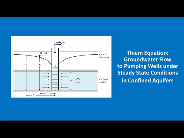
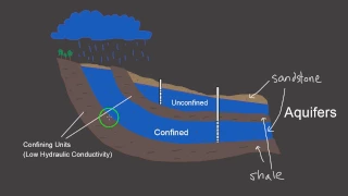
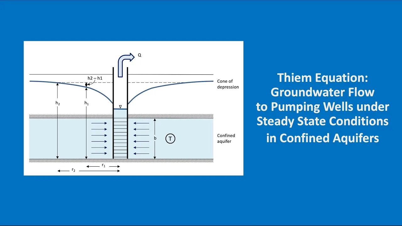
Welcome to Hydrogeology 101 - Pumping Tests. Today I want to talk about the Thiem equation which governs groundwater flow to pumping wells under steady-state conditions in confined aquifers. Here is our little schematic of a confined aquifer, so that's this blue area here which is sandwiched in between an upper and a lower confining unit of low permeability.
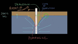
We have a fully penetrating pumping well in the middle and around this well we have a cone of depression in the piezometric surface. So it's not a real water level - you'll only see it if you drill a couple of observation wells into the confined aquifer, and this is the elevation to which our water level will rise in the observation well. If we look at it in three dimensions you can imagine that it will look a bit like this.
We have our well here in the middle, and then we have here an inner radius represented by our first observation well and an outer radius represented by our second observation well. The ground water will flow towards our pumping well from all directions, so it's radial flows coming from all directions towards the well at the centre and you can see it's represented by a few arrows here. .
. and as we go through the inner radius, the groundwater flow will start to speed up a bit because what happens is that the same quantity of water has to pass through smaller and smaller sections of the aquifer. Don't forget that we're in steady state so that means that the amount of water passing through the outer radius is the same as the one passing through the inner radius and it's also the same as what actually enters our well.
In previous videos we talked about Darcy's Law: Q equals KIA, and I want you to pay particular attention to the A part of it, because previously we looked at Darcy's law in respect to sections through the aquifer which had a length and a thickness. What we're going to do now is take this section and wrap it around our pumping well so that the radius is this 'r' here. OK, so basically if you think of this outer radius here it is just a long strip of aquifer, that has been wrapped around the pumping well which is in the centre.
So we can calculate the area of our strip or rather our circular strip by taking the perimeter of a circle: 2 PI R and multiplying it by the thickness B. Now we can combine these two equations. .
. so our area here multiplied by K multiplied by i. .
. will be our discharge. At our outer radius.
. . at r2.
. . our discharge will be 2 pi r2 multiplied by b multiplied by K multiplied by i2.
. . i2 is the hydraulic gradient at this location, so basically it's a line drawn at tangent to the cone of depression at this location.
Now because we are steady-state, the discharge at the outer radius will be the same as the discharge at the inner radius. What I'd like you to notice is that b and K are constants - they don't change. Our aquifer thickness doesn't change.
What this means is that the only thing which is changing is R and I so the distance from the pumping well R is of course much larger at the outer radius than at the inner radius, so the only way that you can maintain the same discharge is if the gradient becomes larger as we approach our pumping well. . .
and this is the reason why we have a cone of depression. As we get closer and closer to the pumping well, the hydraulic gradient has to increase to maintain the same flow. Now our cone of depression is not a nice straight line.
. . it's got a curve to it.
. . so it gets a little bit more complicated and we have to write it in this differential form, which after integration we end up with this equation which is called the Thiem equation of 1906 for steady state flow to wells in confined aquifers.
It's not a complicated equation basically just take two Pi multiply by aquifer transmissivity multiply by the difference in drawdown between two locations - any two locations along our cone of depression - divided by the natural logarithm of the outer radius divided by the inner radius. Often we don't know the exact elevation of our observation wells so what we can do is just take the difference in drawdown. So you notice it was h2 minus h1 here.
. . but we do s1 minus s2 because we don't want to have a negative number.
We just want the difference in the drawdown. So this is our equation if you have drawdowns only. OK, let's illustrate this with a practical example.
Let's go to Kabul Afghanistan and my regards to everybody there who is suffering from corona virus at the moment I hope you make it and then we can meet again soon. OK, so let's go ahead. My first question is how much water can we extract from a well in the lower Neogene aquifer if we want to limit our drawdown in the well to 50 meters.
I should say there there is a deep aquifer beneath Kabul that was studied for five years by a Japanese team paid by JICA. So here is our schematic of the aquifer and basically what we want to know is what is the discharge Q for a drawdown of 50 meters in the well. Notice that will use sw for drawdown in the well instead of s1.
So in our Thiem equation what we need to know is what's the difference between s1 and s2. . .
. s1 here becomes sw and for s2 what we're going to use is the radius of influence of the well at which point s2 will be 0. OK, so our equation simplifies a bit.
It's just 2 pi T sw divided by log n of the radius of influence divided by the radius of the well. Now we know what Pi is. We don't know what the transmissivity, T is.
SW is 50 metres as specified before. Our radius of influence - we've arbitrarily taken a thousand metres. Our radius of a well - let's assume it's 10 centimeters.
. . point 1 of a metre, and to summarise in order to find this discharge for a drawdown or 50 metres, we just need to find out what is the transmissivity.
So earlier I went to Google and I typed in neogene Kabul JICA and the second hit here is the 2011 JICA study on a study of groundwater resources potential in Kabal basin in the Islamic Republic of Afghanistan, and in the executive summary we read that the low Neogene consists of clay, gravel, sands, gravels and conglomerates. it's pretty thick. .
. 252 metres. .
. 159 meters however the transmissivity was very low: only 8 metres squared per day on average. So that's not a lot.
Let's plug it into our equation so here our missing number: transmissivity of 8 metres squared per day. If we plug it into our equation we get 2 multiply by pi multiply by transitivity multiply by the drawdown in the well, divided by log n of the radius of influence divided by the radius of the well, and we end up with 273 cubic metres per day. Question number 2: what does the cone of depression in the piezometric surface look like?
Illustrate with a graph. So this is the graph that we want to make but let's go first to the Thiem calculator which is a little tool I made in Excel, so you can probably recognise our diagram of the confined aquifer here, and if we move down we can see the Thiem equation, and also the key assumptions which are very important. Don't ever forget that the Thiem equation only applies if all these assumptions are correct.
So I've already entered the inner radius its the radius of the well. . .
point one metre. . .
the outer radius 1000 metres, and then we have to add the head of the inner radius and outer radius so that the drawdown here is 50 meters. Now I've just put in 50 and 100, but I could easily have put in for example 0 here and 50 here. .
. it has the same effect. .
. we just want to end up with 50 metres of drawdown at our inner radius. OK, so let's add the aquifer transmissivity.
. . watch this space carefully as I enter the 8 here.
. . enter.
. . and up pops our transmissivity.
This is a label that has a live link to this label field here. Now if we look down at our calculations, there are enough parameters now to calculate the well discharge based on the Thiem equation, and we can feed this back into our parameter table. .
. equals Q. .
. enter. .
. and then you will see that all the other parameters have been calculated as well and it should be the same as what we have here. OK, here is our discharge.
. . you can see it here.
. . and also on the right is a chart of the cone of depression.
Let me quickly go down to the table where it's calculated. We have here a variety of radiuses between our well and the radius of influence and in this column here will be calculated the H number for each of those locations based on this equation here. .
. and from the hydraulic heads we calculate the drawdown. .
. very simply it's the difference between the outer radius head and are calculated head and then these numbers are fed into our chart here. You'll notice that there is a very, very steep cone of depression as we go closer to the well which means that it has a low transmissivity.
In fact if we go here at 200 meters we still have a drawdown of 8. 74 metres. That means that if we're pumping from the Neogene you'd have a quite a big influence on any wells in the area.
OK, let's have a look at our third question: what are the conclusions about developing the lower Neogene aquifer. If we go back to the JICA report they conclude with the potential of groundwater development of the deep aquifer is not high, even for emergency purpose. So I think we can fully agree with this conclusion the lower Neogene aquifer is really not suitable for development as a water supply source for Kabul city, and mostly because you have such huge drawdowns for very small discharges and big drawdowns means high energy costs which means that the cost of the water will become very high indeed.
OK, so that's it for this little video. I'm going to make another one for unconfined aquifers shortly, and I hope that you watch that also. I hope you enjoy this video and thank you very much for your attention!