Lecture 24: Phonons

welcome back uh today we are going to move into lecture 24 and we will be talking about phonons last time we spoke about photons which were fundamental excitations of the electromagnetic field and here we are going to talk about phonons which as we will discuss uh fundamental excitations of the lattice vibrations so uh i'm i have to warn you at the outset of this lecture that this is not a solid state physics lecture so uh i'm going to do my best to introduce you to the notion of phonons but a full treatment should probably be

needed until you take a solid state physics course so i'm going to try to explain to you the basic uh and fundamental principles that you need to get in order to to understand the temperature effect for phonons so in this lecture we'll talk about the einstein model the dubai model and we will discuss quite a bit about dispersion relations so i will remind you what uh the notion about the notion of uh this persian relation and uh you the kind of system that you are going to consider is a system like this where we have

a solid and we consider that each atom in that solid they're all they are connected by by springs at least the closest atoms are connected by springs if they are all the same atoms the springs are all the same and the question is knowing that each spring can can vibrate what are the possible vibrations of this system so this is basically what a phonon is phonon is is a is one of those vibrations of the crystal and there are more than one phonon i'd like to tell you also that we already discussed this a little

bit we looked at the equip when we did the the lecture lecture 90 on the equipotential theorem we already calculated the heat capacity of this system and we found that uh so long as the equipartition result is correct so as you know at high enough temperature and so long as we see the harmonic approximation we found that the the heat capacity per mole was 3r or 3 kb per per atom so we'll see if we can uh the result that we are going to discuss today are going to be compatible with this so phonons let's

say a little bit about phonons uh so first of all the phonons are considered as excitations of the of the lattice of atomic lattice a crystal lattice and the the energy of this those excitations are h bar omega where omega is the angular frequency of those vibrations so of course they are like waves so they do vibrate um so as i mentioned a minute ago the phonons are the quantized elementary lattice waves so when we look at the at the simple harmonic oscillator this is kind of a phonon if you want but there's only one

one vibration for the for that system here we are going to have a collection of them because we have multiple atoms and if you know if you have multiple atoms that means that you have three n degrees of freedom so those vibrations uh are going to be called uh normal mode and the normal mode um is basically the all those modes the list of of possible vibrations that are independent from one another so i'd like here this is where the math is actually useful uh the normal modes are actually obtained from diagonizing uh symmetric matrix

therefore those modes are orthogonal to each other and they correspond to uh to fundamental vibration so i'm giving you all this with that proof but the the points remain because they are orthogonal to each other they are also independent and so long as we stand the harmonic approximation there is no crosstalk between the normal node as you know that's going to be very important when we calculate the partition function since the partition function is different if we have independent system versus interacting system as we have discussed but i will review that again uh we are

going to consider each of those modes as simple harmonic oscillators so with everything that we've learned about partition function of a single harmonic oscillator and um one thing that's very important and in fact this is going to be the the thing that we tune throughout this lecture is how to understand the angular frequency versus the wave vector k so this is a notion that students sometimes have trouble with i'm going to try to explain that to you a dispersion relation is really what's telling you how fast a wave oscillate as a function of its wavelength

as you know the wave vector k is 2 pi over lambda lambda being the wavelength and so so basically what when we say omega versus k we are really talking about how what is the vibrational frequency of a wave propagating in a crystal as a function of his wavelength so this is what we call a dispersion relation and we know for example the dispersion relation we've noticed we've we've seen one so we know the one for photons right we just had um we just had omega is equal to uh ck if i for if i

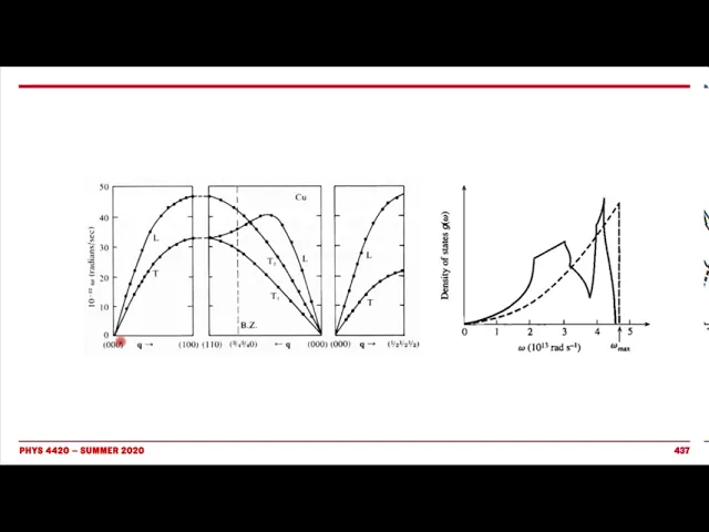
remember well so this is just a straight line right this is this is what we've seen in the previous lecture so we'll see that it's a little bit different here and i'm i'm going to show you two very simple examples where we will calculate those dispersion relations so basically finding the frequency as a function of wavelength um and i also show you real examples uh in this lecture so actually i'm going to start right there so these are these on the left hand side don't worry too much about the right hand side for now just

focus on this and these are um these are the relationships so these are the dispersion curve so frequency that's the function of the wave vector by the way we usually call it q uh when it comes to phonons instead of k when it comes to photons it's just just a convention but you could in principle use k here if you wanted to but we typically use q for for for phonon uh the point is we have those curves that correspond to the frequency as a function of wavelength i'm not going to go in detail about

this notation here uh suffice to say that these correspond to different direction in the for the crystal lattice okay so this is what this is what we have let's not worry about how we get it and i'm going to explain some features the point remains because we we can consider the wavelength as a label so the wave vector q which is the inverse of the wavelength as a label uh we see from this that um we have a certain number of states depending on the frequency omega okay so we go back to what we call

a density of state and i will discuss that in a bit more detail in a second and if you look at the density of state of copper for instance you will see that as a function of frequency you have an increased number of states and sometimes a dip and you're going to have a dip for example when you have in this in this area for example here and then you're going to have maxima and the maxima is when we have flat band because flat band means that for a very tiny interval of frequency you have

lots of state and this is what the density of cedar of course means if it is not clear to you at this point um do not worry and do not uh do not tune out just yet we are going to to describe that in in in a moment for now what you need to understand is that this density of state here uh provide us the priority distribution as we discussed before that we need to calculate um for the distribution of state that we need to calculate the partition function okay now the problem is how do

we model this and we will introduce two methods two historical methods to to uh model this complicated uh curve right here so that's what we are going to do now so that's the reason why i'm showing you this at the beginning of this lecture okay so let's start with einstein model uh so the remember that the model we are looking for is that how do we describe the number of vibrational states as a function of frequency okay so the einstein model is actually pretty as simple as it gets if you want even though it's very

successful it's just to say that the density of state to the number of states between omega and omega plus d omega right the definition of g of the omega that density of state is actually the dirac delta okay uh it's a direct delta that simply is there to say all the the mode they have the same frequency that's what that's how you translate this mathematically so all the mode has a single frequency of course you can argue that it's a pretty uh pretty mediocre uh approximation but you will see that it works pretty well and

that frequency we for now we are going to call it the einstein omega okay we'll see we come to we'll come in a second to explain what that omega should be that omega e should be but we are going to call it einstein omega okay so that's all nice now we know that if we have a solid with n mode with n atom sorry there are three n modes right there three we discussed this already when we look with when we were in the lecture on equi-partition theorem and so that means that we have three

n mode simply because remember each atom has is connected to um it's connected to two tools to uh to the number two okay let's say they are connected to other atoms through the springs as we discussed that and that three of them uh unique spring per atom i know it's six but because they share the spring it's on average it's three per atom um so one thing just to make sure that you you guys are not too confused that actually in in a you know in in a finite solid like this we have three and

minus six mode why because among all the modes there are some that are just translation of the entire system in either x y and z and three rotations around the x y or z axis these do not correspond to vibrations so usually we have three and minus six however we don't worry too much about the six because we are talking about macroscopic solid so n is extremely large even if you have one mole of copper let's say that's 10 to the power 23 n equal and n equal 6 10 to the power 23 the avogadro

number so adding six or subtracting things makes essentially no no difference whatsoever but to be correct the number of mode is really three and minus six we will suppose that those modes do not uh do not interact and are independent so this is actually the an assumption that we will keep using uh for the other model that we will look at and that allows us to calculate the partition function so the partition function of a collection of three and more that do not interact is simply the product of all the partition function well we've discussed

this at detail in details in the past few lectures of course that means that the logarithm of that partition function is just the sum of the logarithm as we have seen a number of times and z k as we calculate as we noted here is the partition function of a single mode and remember what we decided to do is that each single mode is a harmonic oscillator it's just a it's just a vibe an oscillation and this is nice because we calculated this we already know the partition function of a single simple harmonic oscillator is

just the sum of all the boltzmann factor and we know the energy of a quantum oscillator this is n plus one half h bar omega beta and go from zero to infinity so a few comments uh just to make sure that uh just to make sure that you remember this uh here all the frequencies we said are all the same it's it's the einstein frequency that's what it decided to do and uh the one half here is actually the zero point energy okay that means that the energy of the oscillator is never zero so this

is a very simple sum to calculate and we obtain this result that we have seen a number of times already in this in this course one thing that we will need as you know is the logarithm of z uh and then we know the logarithm of z is just the sum of the logarithm of z k and this is very straightforward to calculate the logarithm of this simply the logarithm of the numerator minus the logarithm of the denominator and we can obtain this directly as you know the partition function is very important because we can

get all the other properties of the material of the thermodynamics thermodynamic properties and the logarithm is usually comes into the game so we probably have everything we need to understand einstein model at this point so just to repeat so it's clear the einstein model uses as this the main assumption that all the frequencies all the density of state is actually there at direct delta in other words all the oscillatory frequencies are one single frequency so all the the uh oscillators uh vibrate at the same frequency this is actually a very rough approximation okay however however

because we have the right number of modes this model keep the number of mods to 3n okay it turns out that it's because of this the normalization is right a lot of results that we obtained from this simple model are actually very close to the experiment we are going to let's not jump the guns and we are going to get there so just to just to remind you this is the this plot here the density of state is the one that's actually the experimental one so the full curve and the einstein model simply using a

single approximate all these features by a single peak okay so yeah it looks like pretty rough but this is this is the idea and by the way maybe it's not that bad if we were to try to represent this peak here we'll discuss that in a few minutes okay so let's go back to this we calculated the logarithm of the partition function and now of course we can get the internal energy internal energy it's something we've seen before it's minus the derivative respect to k one over k dt uh this is a straightforward uh derivation

and we obtain this energy here and which can we can rearrange a little bit the the different terms it's not that's not very complicated again and then we obtain that the um the internal energy is going to be equal to this equation here which i'm not spelling out because it's just written written right there now one thing that people like to do is to instead of using the einstein frequency we uh the einstein angular frequency here we actually use the einstein temperature okay uh it's capital theta e and the reason why we can do this

is of course h bar omega is the energy of elementary excitation and kbt is also an energy so basically here we are essentially changing the units between the frequency the einstein frequency in the angst and the einstein temperature it's just that it's it's you would typically use the einstein temperature as you know to move from one to the other you have h bar the planck comes the reduced planck constant and kb the boltzmann constant nothing really difficult one thing that i should also mention from going to this from this equation to this one we move

from the number of particle n to r uh i mean actually we move from kb to r but because we we divided this equation by the avogadro number so that this equation is really a per mole equation while this equation was for n particle this is something we've seen before this is how kb becomes r we've discussed this at detail in details and i invite you to review this if if it's uh if it's a bit blurry in your memory very nice we have the internal energy now we can look at what happens at very

high temperature so this is what we had in the previous slide and if we have a very large temperature we can actually look at what happens to the exponential as you know very large temperature means that the argument here is very small and if it's very small we can use taylor taylor series stated expansion uh close to zero and of course the exponential close to zero is simply the argument plus one right this is the id this is the argument plus one if x equal to zero it's of course one and this is the first

linear term so basically this term here is simply one plus um theta e over t and of course it gets rid of one here so we can obtain directly here that's nice because this is very easy to simplify and we see that when the temperature gets really large this term of course is much smaller than this term when temperature is very large and we find that the internal energy is 3rt which is something that we've seen of course for the equipartition result so that's nice we have the preparation result that's not a big surprise of

course because we are using essentially the same the same framework the only difference is that now we include the density of state but since we are looking at a large temperature uh the distance between the level does not matter anymore so that makes sense that we have the same result but it's always good to check um we can also look at the molar heat capacity so molar heat capacity remember it's the heat capacity per mole right of the einstein solid so we can calculate the capacity as the derivative of the internal energy with respect to

temperature one thing that's important here and it's a question that's been usually asked in a test to make sure that students follow why don't we use a v or p because remember we define the heat capacity at constant pressure constant volume the reason why the reason why we do not worry too much about that is because for solid cp and cv are pretty much the same because there is no there's no much of the energy that goes into compressing the material as opposed to a gas for example okay so that's the reason why we usually

drop the v o p because these are essentially the same so we can calculate the derivative from the equation i had before and the derivative is elementary we obtain this this equation right there and we can rewrite it in a slightly uh nicer way by by writing that x is equal to theta e over t nothing really complicated again remember that this is true for every temperature we don't have we did not take the limit of high temperature yet or small temperature well we are going to do that just now so when the temperature goes

to zero uh that means that x goes to infinity and when x goes to infinity uh this term uh is the largest term so but it's square so but so it's simplified with this so we get n minus x and x square so this falls very fast this is an exponential as you know all the exponential the decaying exponential always decay faster than that any polynomial grows so that's going to be that's going to be uh clear that the heat capacity will fall very fast in fact it falls a bit too fast compared to experiment

and um we will get a better a better description in a minute and the reason why it falls very fast compared to experiment is because the low temperature at low temperature we start to uh to explore if you to visit the low frequency mode in the density of state but those low frequency modes in the einstein model are not very well described because we describe the entire model as a single delta peak so of course when at low temperature we do not expect this to be good on the other hand at high temperature all the

more that basically um ever actually been uh visited and including so this is really an average effect so if the peak should actually be pretty good to describe the the average of the entire the peak that we have in the einstein distribution and in fact at very large temperature so when x equals zero we find that the heat capacity is three r and the heat capacitor is the long protein that we've already seen in a lecture 19. so this is actually the right the right the right limiting case as i said that makes sense because

at high temperature the details of the density of state does not matter as much as the fact that it's normalized correctly which it is for the einstein model with the run delta that's very good uh now it's time to move toward to another to another model which is a dubai model so the dubai model is a little bit uh more advanced i would say but we will see the difference uh in a minute so just to remind you what we did was the einstein model we never actually had to introduce the the the delta because

the delta what came into the sum to the partition function but this is really what we did uh is the fact that the density of state so the number of states between omega and omega plus d omega is just represented by this direct delta and the three hand here make sure that the system is is the the integral is properly normalized in other words we know we have three and state you can argue it should be three and minus six but any so large it doesn't matter okay so very nice so what does the dubai

model do well the dubai model basically says while a single peak is as as screwed as it gets let's try to do a little bit better let's suppose that for the number of state between omega and e equals omega we are going to suppose that all the waves travel at the same speed vs okay which is the speed of sound okay remember q is two pi over lambda as we discussed before so basically what we are saying now is that all the all the modes all the the phonons go uh travel at the same at

the same uh speed okay and that means that if you write that in in math that means that the frequency the angular frequency is vs speed of of sound times q so let's try to take a moment here first of all the units are right this is this is frequency so it's a per second it's q it's two pi over lambda so it's a per meter if you will so this velocity is meter per second so meter per second times meter minus one gets get the frequency so that's good so basically saying that all the

waves travel at the same speed v s simply means that the dispersion relation is omega is equal to v at q so basically it looks very much like what we use for for phonons for photons but in that case we have the speed of light so it's going to be a straight line in the omega versus q plus okay so is that better well we are going to see that in a second so first of all we the advantage of this is that we can now calculate the density of state as a function of q

and in fact we've done it already a number of times uh this is exactly the same as we did in the previous lecture for pronouns but let me try to re-explain to you a little bit here uh the the number of state between q and q plus dq so again q is the wave vector is going to be the volume of the shell the spherical shell so again the volume of the spherical shell is the surface of the spherical shell four pi q squared times the thickness okay and we divide that by this by the

volume of that each individual state takes which is two pi over l cube in three dimension and why where where did where does that come from well it comes from the fact that the waves are confined in a volume of length of a cubic volume of length of side l okay so this is something we've seen a number of times it's very important to realize this here when we did photons we had a factor of two because we have two polarization here we have three a factor of three because we have three possible uh uh

possibilities for the waves which is one longitudinal so along the the direction and two transverse superpower decay the direction so it's a factor of three here very good so basically this equation if we say that l cube is equal to v as always we find the density of state to the number of states between q and q plus d cube given by this formula now we know in the partition function we usually sum over energies and what we know is uh usually energy is h-bar omega for this for this uh elementary excitations so that's what

we are we are going to look into so if we consider that the frequency is v sq okay so it's nice because it's linear we can transform this density of state per per q if you will per per wave vector into a density of state per frequency and this is what we obtain uh this is really fairly straightforward uh you have a cubic term in q q square you have a vs vs square coming from here vs coming from here so that's uh that's vs cube okay that that allows me to to make the replacement

that's that's actually pretty straightforward because you can see from here to here that's nice because that gives me the density of state this is what i need to calculate the partition function remember partition function is going to be obtained from from an integral over all the boltzmann factor for which we have to include the density of state or basically the degeneracy that's what it does so just to be clear this density of state now gw is a quadratic term in omega so basically it's a parabola okay it's a parabola right here okay it's a parabola

but we have to make sure that that parabola is normalized properly remember we need to make sure that we have three and state in that density we don't want to create state that don't exist and uh i'm maybe i'm jumping a little bit ahead of the next slide but the point is that that means that when i integrate this i need to obtain three n and that will force me to stop at some point when i obtain three n at the point where i have to stop is called the buy frequency so the capital d

here means that the buy frequency so this is basically all the way when i stop integrating this is what we obtain and this the by frequency is obtained so mathematically what i just said you integrate this function until you found that you have 3n remember it's a density of state so the number of states between zero and the by frequency has to be three and for proper proper normalization since i know i have three instead very nice so now the red curve here so remember uh the red curve represented the bi model okay so what's

interesting here of course is the fact that uh this is the the experimental result for the density of state for copper and now instead of representing this by a direct delta as we did for with the einstein model we are representing this with a parabola it is still pretty crude you see you do not represent those features or this dip but i would say that in general especially at low frequency you're doing a pretty good job okay doing a pretty good job so you expected the buy the buyer model to works well especially for those

low energy excitation which would occur at low temperature so hopefully at low temperature we have about the description and we actually do we are going to see that so now we have everything we need to calculate the partition function and from there we can calculate the energy and the heat capacity let's do it so we have this density i explain a minute and we have to go to the buy frequency so we can calculate this is very straightforward calculation this is basically telling you until which frequency you have to integrate same thing as we did

before for the hunch for the einstein temperature we can also introduce the buy temperature with simply a change of units if you will from the uh the buy frequency and again you can change the units by h bar omega and k dt and so you obtain the temperature thereby temperature so in fact it's very important the by temperature is basically close to what we said the maximum frequency that we have to take into account right it's it's until when we have to stop to get 3n so this is a good property of material uh so

uh there are examples and it's taken from the from the textbook so from the blundell and blender textbook and we see that different materials will have different dubai frequency and this is actually quite interesting here because even though this is not a temperature you measure you know you do not measure this temperature with a thermometer it represents the highest frequency that you can have in your system and of course the highest frequency means that you if you have a stiffer system like like a for example uh diamond is a very stiff material and as compared

to neon for example which is which is a uh which is definitely not a stiff material because it's essentially very little interaction between the particles so you see that uh these properties provide this dubai temperature provide a very interesting uh way to see uh what kind of chemistry happens in the solid in the in the system uh going from a gas to to a solid basically again i'd like to say that this temperature has nothing to do with a temperature you measure it's really this temperature from the model of the dubai model but it's very

close to the maximum frequency of the phonons that we have in the system okay good now as as i said a couple of minutes ago we are going to calculate the internal energy and we are going to calculate uh the heat capacity so the internal energy again same as always exact same equation as we use for um for the for the einstein model is just that the density of state now is not a simple direct function uh direct distribution but instead is this is the one we just calculated uh and uh uh we have not

yet introduced it here we're just playing a little bit with with these these equations and if we remember what the the density of state is and the by frequency is you can reintroduce those properties in here and obtain finally the logarithm of z okay so this is a little bit cumbersome it's the mass here looks a little bit uh not as clean as we would like it to be but uh [Music] we are going to make it and so we can certainly calculate the derivative of this the minus the derivative of this to get the

internal energy and we obtain that the internal energy is obtained by this equation here where we have not performed the integral yet we are going to do it when we calculate the heat capacity this is the internal energy this is how we get get it the only complication is is that is the bookkeeping to make sure you don't lose anything when you do the math but in terms of the approach to start from the partition function all the way to the internal energy is the same as what we've done a number of times in this

in this course so the heat capacity is something that we can measure directly right so it can can be calculated from the derivative again no p and v subscript is necessary for solid and we obtain uh using the internal energy that i had from the previous slide that's why i will produce it here then calculate the capacity the heat capacity as the derivative with respect to temperature and we obtain we obtain this this equation that's not necessarily good looking it doesn't really matter what is a good looking equation anyway but the point is we can

analyze this and we can analyze it by uh simplifying a little bit denotation by by writing x equals h bar beta omega beta okay is one of the kbc nice now here is the result that we obtained when we when we plot c over 3r we already know that the einstein model does indeed converge are at height at very high temperature and we also know that it decays as i mentioned to you well i just said that to you that it decays a bit too fast okay it is a bit too fast because we do

not represent the low frequency very well now the dubai model seems to not decay as fast as the einstein model and we will see that this behavior is actually the appropriate behavior uh we can actually zoom here and do the calculate actually represent the logarithm of this uh the the log scale of this and then we see that indeed at very low temperature uh we find that uh and here the the the dubai uh temperature and the the einstein temperature are chosen to be the same you see that the by temperature uh behaves like uh

like a power of t right it's it's a it's a loglock scale so a power is going to be represented by a straight a straight line while the the einstein model details exponentially as we have seen uh and therefore it was represented by by this kind of curve so einstein the einstein model it is actually too fast compared to experiment which is very close to the buy model so let's try to see this analytically a little bit uh so this is the formula i already showed you five minutes ago uh let's let's look at the

the two limiting cases uh of uh high temperature and then high and in low temperature at a at high temperature um this the beta gets gets to zero right it's it's uh one one over kbt uh so we get x equal to zero so we know that this is very close to uh this is very close to x right because e to the power x is one plus x so that means i have x left x square x x 4 divided by square and of course e of x close to x equal to 0 is

uh is indeed 1. so i obtain this this formula here that we can easily integrate right we have x square so that's x cubed over three uh calculated that the the the the by uh the by uh x if you will and we obtain three r which again is the same result that we found for einstein and the doula and again that's not really surprising because all those models were using the right uh description with the right number of modes remember that the dual operating and the equal partition theorem were based solely on the fact

that we were taking into account the right number of modes that come from the partition so we did this with both einstein and dubai and the details of the density of said does not do not matter anymore when we are we are at very high temperature okay this is a reminder now low temperature is a little bit more interesting at low temperature we can we can calculate the the how this this is going and we can actually use the user use a formula uh why why can we use uh uh formula from the table because

now the integral is actually an integral from zero to infinity because at very low temperature x uh goes to infinity right because beta is one over kbt so at very low temperature whenever kvt goes to infinity so x goes to infinity and this integral can be found in in a table of integral and we obtain that here the result you obtain is the the heat capacity behaves like 1 over x to the power 3 e which is of course means that it's the temperature cube which is exactly what we found on the previous slide and

this result is actually pretty close to to what you expect to have experimentally much better than the einstein model okay now let's try to let's try to do even better um i like to spend the last few minutes here to try to explain to you where we can understand those disperse this dispersion relation so again just to remind you the dispersion relation are going to give you the frequency as a function of wave vector so how fast wave oscillator is a function of its wavelength that's basically what it does now we are going to use

we always with the simplest model which is a one single atomic chain of atoms that are all the same all the same mass all the same spring constant and so the most important thing to understand for the entire uh for the entire discussion is this this entire discussion is based on newton's law the second law and we are going to write u of n as being the displacement so along x okay the displacement of an atom of atom number n um from this um from its equilibrium position okay so so dot dot means the acceleration

so so mass times the acceleration let's say of this atom is going to be equal to the force on that atom right this is the second this is the newton's second law well the force on that atom is related to the hooke's law from the spring here and from the spring here so the spring the force is of course as you know minus kx okay depending on how you you look at your you put your axis you place your axes the point remains is that if what matters is the difference between those two displacement indeed

if the two displacement were the same the spring will not be compressed or elongated so there will be no force so what really matters is the difference between these two so there will be an interaction in fact this is this one and this will be an interaction from the spring between n and n minus one this is this one so the difference how how much the the spring is compressed or elongated and of course a force coming from the next one because this is the only the way we do it if you understand this you

basically have understood the whole thing because what it means it really means um it's it's it's uh it's the newton's law okay with the hook's law for the for the spring and of course we can rearrange the term and we obtain this k is the uh force constant for a single spring yeah very good so we obtain this and what we'd say is that we would like to try a wave-like solution for this so we just say okay the displacement along this chain is going to look like a wave okay this is what i'm looking

at and now the advantage of causing a wave equation as you've seen in your introductory physics course is that there is an oscillation uh oscillatory behavior because it's uh uh which is related to the separation a between between the atoms and also an oscillatory behavior in time uh which is related to the angular this angular frequency here so this is the typical thing that we look and we look at the propagating wave so we we can just um substitute this solution in here and see and see if we can do it if we can if

we can solve it in fact if you do this the the advantage is that things get pretty simple because the second derivative here is going to respect time right is what the dot dot does we obtain uh i omega times i omega okay so that's minus omega squared times m that's what obtained here on the right hand side times the exponential of course which is going to to to simplify and then we have to calculate this thing here and these things here just depend on n which means that we are moving away from one lattice

constant a and one one one away to the right and one away to the left here and so we obtain this equation and basically believe it or not but it's done because now you know the euler relationship for the complex exponential and you see probably a sign qa here actually the two sign qa and you oh a cosine qa because it's a plus yes uh yes indeed so 2 cosine qa sorry about that so we obtain that and and we we see of course that we rearrange and we obtain an equation like this which is

a relationship and it's what's important it's a relationship between the frequency omega and the wave length q indeed k m and a are constant the parameters for the problem it tells you the mass of the atoms the strength of the of the spring so the strength of the bond if you will and a which is just a lattice constant so basically what you have here is exactly what i advertise at the beginning of this lecture as being a dispersion relation which provides you a relation between the frequency and the wave vector so this is very

nice because that simply imposes that condition that if you have a given wave vector you must have a certain frequency so it tells you this problem tells you if i have a wave of a certain wavelength it has to oscillate at a specific frequency okay so this is what a phonon dispersion relation is uh and you can plot this you can plot this uh you can plot omega as for omega versus q right sometimes omega versus k but as i told you we use q for phonons typically and what we what we found what we

find is that of course here we recognize the the square of half of the of the angle of the uh the square of half of the of the angle under the body it's very basic trigonometry but the point remains that you obtain this very nice curve that looks outside okay um this this term here is this this zone where q exists is called the real one zone but we are not going to worry about that in this course because it's not necessary for what we want to do the point remains though when q is very

small and this is called the very long wavelength limit remember q is 2 pi over lambda in one dimension right so that means that a long wavelength very long wavelength limit means a very small value of q and in that case cos qa is almost equal to uh yeah it's also almost equal to one my one uh minus qa okay so that means that when we get here we obtain that the frequency is actually going as a straight line if i'm not mistaken actually i'm sorry this is the the the taylor series is of course

not one minus qa it's one plus q a square over two right uh sorry about that so so we obtained this result and we find that at a very long wavelength 1 minus qa by defining the taylor series of course qa as a independent terminal the quadratic term means that omega square is proportional to q a square in other words this is a straight line so very close for the very long wavelength we have a straight line but remember the straight line the frequency as a function of of the wave vector straight line is the

by approximation okay so the y approximation is actually this term here which is nothing else than the straight line so we have something that looks very much like the long wavelength limit looks looks actually uh it's actually exactly correct we are missing this of course but all the low energy excitations are very well described and this is the reason why the dubai model is so good at uh predicting the right heat capacity at low temperature and of course this is not the case for the einstein model i just like to show you here a little

plot for those who to understand a bit better so the largest wavelength you can have in a solid of length l is that you like this longer wavelength means a fewer oscillation then as you increase the wavelength you decrease the wavelength and you get to a larger and larger wave vector you obtain something that's more and more and more oscillatory in space so this is basically the long wavelength limit and as you move forward you have a larger you have a smaller and smaller wavelength so a larger larger wave vector so this is this is

how you do okay so just to go back uh this is this is these are the the type of experimental data and actually and theoretical data that you could obtain to get the phone on uh the relation the the the dispersion relation uh for copper for example and as i said before we i already showed you this picture before this is a bit more complicated than a simple chain of atom but you can represent very well those straight lines close to zero okay the straight line and we actually call them the acoustic uh acoustic branches

because uh they correspond the the the good velocity that so the the the dispersion relation correspond to the velocity of sound in that material so this is this is what we do these are the the actual band structure we call them so the dispersion relation for an actual system uh as measured by uh inelastic neutron scattering uh and so this is the density of state that we were working with and you can see that the bi model is pretty good too uh this is this is what we've done now it turns out that in in

in reality and this is something i'd like to mention here so that you understand that the einstein model is actually useful in some instances as well it's not it's not just that the dubai model is systematically better than einstein the point is in in uh very often we have more than one atomic type so the next exercise to do as i just you can write uh newton's second law uh for this problems well now you have two types of of masses you can even use the same same spring if you want actually they're all the

same obviously because they always joined the two i mean a big m and small m and you can you can actually solve this uh same way as i saw five minutes ago and when we do that you actually start to find mods that are in addition to these modes that we've seen before right sign the exact signs and and almost a straight line close to the long wavelength you also have another mode here which is called an optical mode and an optical mode is actually correspond to this branch that does not go to zero at

q equals zero and actually corresp the reason why they are calculated called optical mode as opposed to acoustic mode is because they correspond to the oscillation of a dipole moment and the oscillation of a dipole moment as you know can interact can couple with an external electromagnetic field and therefore they can be optically excited okay so this is the reason why they are here and just as a reminder the acoustic mode corresponds to this propagation of sound in this system that corresponds to a to a finite uh sound velocity even for at the long wavelength

limit so i'm not going to describe this in detail again this is more for a solid physics course uh i would be happy to provide more information i'd like to show you an animation of this so that it's a little bit clear what we have uh this is something i obtained from physicsanimation.com on youtube and i'd like to show that to you so this is basically we have a chain you have to consider that it's a chain we just show three of the atoms in the chain they have two different masses so you see what

happens is that um you can see that this is these are here the acoustic mode these are just moving or this is also an acoustic mode where the two big masses move in out of phase compared to the small mass doesn't move and here we have uh a change in phase between the different different mode and this change in phase can actually induce uh correspond to the existence of a of a dipole moment uh and uh that's why they could call the uh optical mode and they can be excited that way so this is this

is something that you can you can easily obtain from the analysis of the band so now we may wonder about the the bi versus einstein model and in fact we are not surprised that the buy model is so it's so good at the low temperature uh because it represents the the the low the the low temperature behavior in other words the the low excitation behavior the small frequencies which correspond to the uh to the acoustic mode and we we have we've seen for the simple model of the atomic chain that actually the dubai model is

is essentially exact at very low frequencies as very large uh wavelength now you may say that the einstein model is not so it's not so good but in fact the einstein model represents very well those kind of peaks that we have and these peaks correspond to the flat band in the band structure of the the dispersion of omega versus uh versus q uh how do i know it's a peak well because if it's a flat band that means that even a small change in uh frequency correspond to the derivative if you will of the of

the band which is corresponding to the number of states is very large it's it's essentially infinite infinite so that's very well represented by those sharp peak which we have in the einstein model so the einstein model will be will be pretty good for the for the optical mode so this this concludes this uh this screencast on on the phonons uh the vibration of the lattice so a phonon is a really a quantum mechanical excitation of the of the vibrations uh we've discussed both the einstein and the bi model the einstein model course just states that

all the phonons have the same frequency it looks like a like a crude approximation but it works it works actually pretty well it's actually not so good at low temperature where the the heat capacity is predicted to to decay exponentially fast in the einstein model even though the experiment shows that it decays as a as t to the power three and uh this small the model from dubai uh solved that issue by uh imagining that the frequency of of the mode changes linearly with uh the wave vector and of course the relation of proportionality between

the two is the is the the velocity the the velocity of sound so we've seen all this and we see that in both cases uh the saturation at high temperature is correct which is which is simply simply comes from the fact that we have the right counting of the mode and we've seen that uh even though the band structure so basically the dispersion relation between omega and k and and q really for phonons can be more complicated than what the dubai or the einstein model represents the the limiting case are actually pretty well described in

in in the in in the case of the dubai and uh the bi model follow for low temperature thank you and see you at the next lecture