Build an LLM from Scratch 3: Coding attention mechanisms

Yeah hi and welcome back everyone to chapter three coding attention mechanisms so this is a supplementary coding a long video for the build a large language model from scratchbook and here I'm trying to walk you through some of the code examples to explain what attention mechanisms are and what role they play in the large language model this is actually a very technical chapter maybe the most technical chapter In the book because it's similar to implementing the engine of a car where the engine is the most complex and the most technical aspect of a car in

my opinion so but it's also very important topic because it helps us really understand what the llm is doing and why llms are let's say different than um yeah other types of models for for instance the Transformer architecture introduced um yeah this self attention mechanism that we are going to code in This chapter and it's been yeah very transformational in terms of yeah developing these large language models and also in the grand scheme of things just to take a step back here what we are trying to do here in this video or in general what

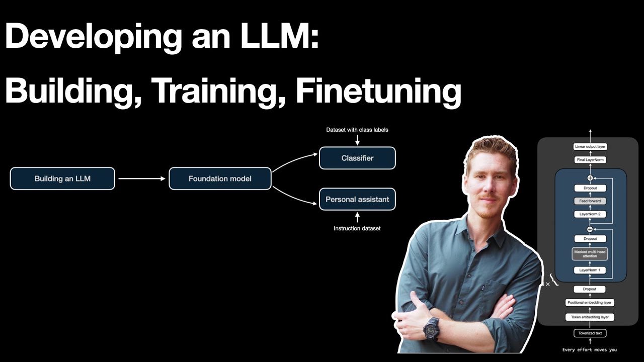
I'm trying to do with the book is to help you understand how large language models work we are going to build a large language model in the next chapter actually and then we are going to train it in chapter five but we Are still you know keeping things more self-contained and small uh yeah for educational purpose purposes this will be a fully functional large language model however it's more on the smaller scale compared to let's say the latest um chat GPD models so personally how I would um see it or compare it is that we

are here implementing an llm that is more similar to an old Ford Mustang for example from the 960s it's a real car it drives however it's not the latest and Greatest car it's not like uh a Ferrari which has been engineered with with uh Millions if not billions of dollars um a lot of expensive Machinery so this would be a car I would say that is impossible to build by a a single person you need a really a big um team for that or a team of Highly um yeah professional experts and you need also

a lot of high Precision Machinery where with this old Fork Mustang you might know that it is possible actually to maybe not build the Whole car but to restore it and to fix it by yourself so if you're interested in cars and so in that sense the llm we are building here it's not a high performance car it's more like a simpler car that we can work on ourselves however it still helps us understand how cars work if we building this simpler car and the reason why we're doing this is we can do it by

ourselves without having to spend millions of dollars on let's say GPU Compute to train a large scale model however anyways the the methods we are going to introduce here are the same so there's um Lots we can learn here and in particular we're going to start here with Section 3.3 attending to different parts of the input with self attention where self attention is a yeah a mechanism to parse the input data so for instance if I go to the chapter itself just to show you where we Are in the grand scheme of things of this

book or this video series here so in the first um chapter we talked a bit about setting setting up our python coding environment and then in Chapter 2 we talked about the data preparation and sampling so here we um yeah downloaded Text data and we formatted the text data we we tokenized it and we set up the pych data lers and we are going to use those later when we are training the llm now we are implementing this attention Mechanism one of the core parts of the llm and then later on in the next chapter

we will be implementing the llm architecture so if I go further to um chapter 3 or I'm already in chapter 3 if I go further to this um figure here this is an outline of the topics we are going to cover in chapter 3 so they are all centered around the self attention mechanism however we are going to approach this step by step first we are going to start with a simplified version Of self attention just to highlight the big picture concept then we are moving from the simplified self attention to the real self attention

mechanism and then we are going to add on specific things that are used currently in the decoder uh llms the popular types of llms and that is causal self attention so this is the concept of causal self attention and then we're going to take it one step further and Implement multi-head attention which is Essentially a more advanced version of causal attention but we will see exactly what that means later on right now in this section in section 3.3 we are going to be focused on this simplified self attention to introduce the concept of self- attention

gently so the reason why we are actually developing self attention or why we care about it is to address a shortcoming that other types of neuron networks had so I don't want to go over all the details here if You're interested you can yeah maybe read the chapter in it entirety but um The Main Idea here is that previous types of architectures for example recurrent new networks when they translated from one sequence to another sequence for for instance here this would be German to English translation what they had to do is they had to memorize

uh state of the input so they were reading the whole input and then before they could generate the output They had to yeah they had to kind of save um summary or like a latent representation a condensed representation of the input and then using that input step by step generating the output if you are not familiar with recurrent new networks don't worry about it it's not really important for the remainder of this chapter or this book at all it's just I'm mentioning it here for I would say completeness for those who are familiar with um

RNs now what's important though is that here the short coming is when you translate text from one language to the other and you can't really look at the full input sentence you can only have like this intermediate State you might lose information and then it leads to an um unoptimal or suboptimal translation so the idea in self attention is for each step when we generate text so whether we translate text or whether we answer questions we get information from A text or we do anything with text really where we generate text at any time we

can look at the whole input so that's the core idea of self attention so for in for instance if we have um a translation task and we are translating the next token so um this is a German sentence and this would translate into can you help me so if we here we generated the first output now we are here translating the second output at each step even though we are at the Second output it cannot only look at the previously generated token it can also look at all the other input tokens so it has access

so there's a mechanism to access all the input tokens that we have provided as the user and what's more important even is that we give it selective access so um for example in this case when this sentence is translated into English it's looking at all the input sentences but I try to visualize it here with these dots each Input token has a different importance for example this first word has a medium importance and these two words have a very small importance very small dots here where um yeah this token has a relatively High importance because

it's relatively important for translating this particular token so if you know German do is the German word for you so in in this case this is actually a very important word for translating this word and so here we are assigning higher Weight we make this token more important and in a similar case um the llm yeah is doing this automatically so it's assigning these important weights to to the different inputs and these important weight or importance weights are the so-called attention scores and we are going to yeah compute the attention scores and sometimes also um

called the attention weights but there is actually a small distinction between attention scores and weights that we will get to Later on also um in this video so this short story here is that when we are generating text at any time we can reference the whole input text if you as a user you ask a question give me the mo most five most important facts of my input document the llm at any time when it generates text it can reference the whole input without you know having to store an intermediate representation so it's it's actually

a very powerful uh Mechanism and so yeah in the grand scheme of things so what we are going to do now is we are going to implement this self attention mechanism before in the previous um chapter 2 video or videos we covered the pre-processing steps now we are assuming we have already processed our data and we are jumping directly into this self attention uh module and then later on in the next chapter we will be implementing all the other parts that go into um yeah Llm so one more figure before I go to the code

example here is a summary of what we're trying to accomplish with a self attention mechanism I mentioned this referencing of all the input but on a more like Zoomed In level what we're trying to accomplish is we're going to yeah we are going to transform the inputs into an different type of representation so in chapter one what we did is we took an input text for example your journey Starts dot do dot step let's say this is an input uh sentence that I truncated a bit here for um brevity so we can fit it onto

a figure so if we have an input text like this remember from the previous chapter we are tokenizing this and then we are converting the token IDs into so-called uh yeah Vector embeddings so embedding vectors and each Vector here just for Simplicity has only three values so we talked about this more in the previous um chapter 2 videos so Where we have a vector representation and now here what I'm showing you is the vector representations of all the inputs what we are going to do now is we're going to consider one of these inputs that

we want to transform into a so-called context Vector it's it's called context Vector because this Z here it's also an embedding Vector but it has the information of all the inputs and so this is if I scroll up a bit it is kind Of connected to what I told you earlier here so when we generating this output token so this specific token it has information about all the input tokens it's actually a weighted sum over all the input tokens so you can see that this one is more important but all of them are involved into

in generating this one here and so when I scroll down again this is what you can see here we have all the inputs here and they are all involved in Generating this output Vector here they have different importances though so um here these Alpha values um Alpha 21 22 23 and two t they are all different weights and this is a measure of how how much of this input Vector will be represented in here so it's maybe a very mathematical um concept it's a linear algebra Concept in a sense because we're going to yeah compute

a DOT product here but um you can yeah maybe we will see in the code maybe it will be more intuitive Once we look actually at the code but so this is The Big Picture level we also one more thing I should say is we are going to focus on the second input so here X2 so X2 is the focus here and this will give us the context Vector with respect to this input all the inputs play a role here but you you have a specific set of alpha weights so you can see there always

a two in here 2 1 2 two 2 3 and 2 T So this means this is the weight of The first input with respect to this one and this is the weight of the second input with respect to the second input that's why it's 22 and then it's the uh weight of the third input three with respect to the second one and so forth so this context Vector is specific to this second one here why it's the second one it's just because I chose for this example ultimately we are going to do it for

all of them so if I go up one more time here here I also picked the second One and the second one looks at all the input tokens but this is also true if we look at the first one it would similarly also look at all the input tokens or the third one and so forth we just have to pick one now for the example because otherwise if we you know start picking multiple ones it gets too complicated we will get to that later because ultimately we do this computation so so we do this computation

here for all um yeah for all the vectors but to keep it Simple we are going to focus on x2 as the reference and the reference is also often called the query so let me actually go to the code and then we can actually look at this in a more um concrete way where it's maybe a little bit less abstract and maybe this helps with understanding what is actually happening here so let me copy a tensor here I have so we are going to use tensor flow again and so this is the Complete sentence similar

to the figures I showed you so your journey starts with one step this is my input tensor and each row here is the embedding Vector corresponding to this token so I'm for Simplicity assuming each word is a token but you know it could be a bit different it could be um split into two tokens depending you know on how I tokenizer works and yeah tokenizers was a topic in Chapter 2 for Simplicity we are just assuming each token is one word and then We have this threedimensional input um yeah Vector embedding for each of these

words so going back to the figures one more time so here uh I'm showing you so here this is if I go up one more time sorry here this is the complete let's say procedure we are going from from inputs to this context vector and we have these intermediate weights but we don't know yet how to compute those so we will take It step by step so we are going to break this down into smaller steps that get us to this context Vector so the first step we are going to take is we are going

to compute these intermediate values so um before these Alpha values I don't want to scroll up again but the alpha values they are the so-called attention weights before compute the attention weights we call the we compute the so-called attention scores which are an yeah non-normalized or unnormalized version Of the attention weights the attention weights will come later this is more like a one step towards these attention weights how they are computed is by Computing a DOT product between an input and each value here in this sequence again like I mentioned before we are taking uh

example two X2 as our query and then for this query we are comparing it to each yeah to each of the inputs here and so one thing again I want to highlight Is we are talking about a simple self attention mechanism later on we will talk about the real self attention mechanism but you know to keep things um I would say step by step and at least making it a bit more yeah approachable I wanted to start with a simpler version because we can always make it more complicated later on but I think this nicely

highlights like the idea behind it so how we compute these values is by taking The dot product between the two and in linear algebra the dot product yeah it gives us um a sense of similarity it's like it's a measure um of how similar two two vectors are essentially I mean there's also there are things involved like um yeah uh taking the vector Norm normalizing the vectors length normalization and so forth but for Simplicity uh we're not doing that we are just Computing the dot product and you can think of it as a way to

measure The similarity between um two vectors so um if I scroll down um yeah let me just go to the code notebook it might be easier so we have now this input tensor here and so this input tensor contains 1 2 3 4 5 6 we're going to focus on one at a time so let's consider as our input Vector let's call this the input query we are considering let's say this one so I can also reference this as inputs or let's let's take the second One because that's what we had in the figure right

if you recall here we have X2 so we are going to also use X2 here and X2 would correspond to the second row because Pythor python is um indexed one so X2 would be the second row 01 yeah um okay so this is our input query we can print it out there we go this is our input query and we do the same thing now considering a different Vector let's just choose the first one here so let's Call this um input in input let's say zero or input one because then we are consistent with this

number it's maybe more intuitive and so we going to call this inputs zero input one so this is the the vector we have here now what we're going to do now is uh a menu ual approach so we're going To compute something here that is taking the element element wise oh we multiplying the vectors um element wise so if I do just you know Brute Force by hand just to illustrate it we do we multiply the first value with a second value here then this value times this Value Plus this Value times this value and

so we get this value out here so this is um yeah the essentially the this Vector do producted with this one and there is a nicer way to do this in pytorch we can do actually torch Dot and then take this one and this one and we get the same value as you can see so this is a so-called dot product that's what we're doing here and now Yeah we could do this actually for all the different inputs here we only did it for the first one but it would be a lot of work right

so we have to either write it like this or this for each one so what we could do is we could actually write a for Loop so if we do a pytorch or let's do a python for Loop first if I do a python for Loop just copied it here so what we can do is we can say for each element in um my inputs Value we are going to we have a result here and we are going to add them to it so it's essentially what I I've been doing here so for each element

so if I print it out for element in inputs zero let's do like print element so it's for each element here right and then we have um index which is a different way of accessing this so this should not change if I do It like this oops uh iterated over one D tensor oh I forgot an enumerate I think so I'm just idx is just a position so this is the same um still the same here you can see we are just iterating over it but why I'm using the index here is that I can

now do the same thing for the query so we have this input query right so I can now also Index this one so I let me change it So it's nicer or let's let's just leave it like it is so here I can now multiply those two and then let me just print them so I have these and then I can actually sum them so one way would be uh let's do starting with zero and then let's just add them up so we're adding them up um oh Yeah and then let's double check results so

you can see what I've been doing here is the same that I've been doing here but now I can do it for all the different vectors right so I can go through those uh actually one second I should probably use a variable here otherwise we will get always the same results let's do I and I so we can change the vector here so the vector 1 2 3 4 5 6 and so forth so this is the First one that should be the same that we got before then we can do the same thing with

the next one another one and so forth again this is still a lot of work right so one way to make this actually easier is to use the dot products right so I could technically go in here and do um then I don't need that one then I could do this um let so we don't need this also then just Making it more efficient so I can do inputs I and input query like this so we don't need this one but see it it doesn't change so it's the same as before we are just replacing

this manual summation with the stop product and if I do the zero it should give me this one or this one basically so this is one way we can automate this now going one step further this code here what it does is It's doing the same thing except now we are going to do it for all of them all at once instead of me having to change this here like this all the time we are going to have a for Loop that does that so for each input XI so the I here for each I

in this collection of inputs we are going to compute the do product with a query so we call that input query right and we're going to store them in This output tensor because yeah it's one so in pytorch or sorry in Python we could use a list and append to a list but in um pytorch we have vectors and tensors and they have a fixed size so it is possible to extend those but it's very inefficient usually tensors are a fixed size so we have to for efficiency say how big our tensor should be and

so here we are saying it has the shape um six six because that's um how many rows we Have 1 2 3 4 five six so that's what we're doing here we instantiating this and then we are filling in the values that we got here so if I print this you can see these values here are the same I'm getting here so if I have a two zero 1 two so this is this value here right and so if I want to get um 0 1 2 3 this value this is the same as putting

a three here you can see these are the same so all we have done now is we have made this a bit more convenient we use This torch dot yeah method instead of us doing this for Loop manually and filling in the values so going back um and by the way I was a bit I skimmed over this but I think there is a typo here um so you can see these are the same values this should be actually correct in the pdf version because I'm 100% sure that this uh was fixed or I fixed

this so I have to contact the Manning layout team to also update this here in this website version and um yeah so if you're a bit Confused why these are the same they shouldn't be the same so they should actually be different values pretty sure in the print version it's correct and I will just contact the Manning team to also yeah update it here anyway so we have implemented this now so we have these these values so these values here are the values you are seeing here and yeah for visual purposes I truncated them so

0.9 really refers to 0.95 and then 1.4 corresponds to 1.4 here so instead of rounding them I truncated them because then I thought it's easier to to identify them here because otherwise it would be 1.5 and then you would be looking here and where's the 1.5 here right so that that's basically why um yeah why these numbers are different they were a bit too large or too long to have them here in the figure so I just truncated them okay so we have done this step now We have these scores now the next step would

be going from the scores to the attention weights and again the whole reason why we are doing that is it's a measure of similarity how yeah how similar is the input to this query so if I look at these values here um or maybe it's easier to look at like look at them here you can see this is a higher value than this one so 1.4 is higher than 0.9 so one might say oh Journey here the second Word journey is more similar to the input which happens to be also Journey so it's it's a

way of saying oh they're more relevant to each other than this one which is a bit different now these values later on there are weight values involved uh so here we are talking about attention weights but there are um parameter weights like new network weights that are going to be trained in in chapter 5 and then these scores are optimized for the task at hand so Sometimes depending on the input one word is more important than the other and the network will learn how to recognize which word is important with its weight training basically so

here you know it's a very simple attention mechanism like I mentioned before so I wouldn't take these values too seriously it's more for highlighting what is the actual computation that is happening in in the attention mechanism so what we have done so far is We took the dot product between an input and each of the other inputs we got these scores now we are going to normalize these scores so that they sum up to one so it's it's a normalization and this is yeah done to so that we don't get crazy large numbers and it

helps also with the optimization process to have smaller numbers it's more like a cosmetic thing to do and so there are different ways we can normalize so you probably yeah would think of the most Intuitive way of um dividing each score by the sum right so that would be one way to do it so if I have let's say attention weights to let's call this temporary because we are going to introduce another method later later so attention score is two and then what we could do we can uh just divide this by the sum and

yeah probably you already know what happens now this will be then um giving you the normalized scores you can see that and They are all smaller than one but what's more important is of course that they now sum up oops sum up to one so just making the properties a bit nicer for normalization purposes and there's one actually more common way of doing that it's the so-called soft function so I'm going to define the soft Max function here myself and um this is something I wouldn't use in practice because it's not very stable numerically for

yeah um certain values But just to illustrate it it's basically um exponential of the input divided by the exponential value oops and then similarly the the sum so this is similar to what we've done here so this will also give us normalized values so we call that let's like this call that attention scores two so the reason why I'm calling this attention scores two is that it is with respect to the query for the second Input token so that's why why the two we would technically do that for all the other ones too but we

would have to change the query and that is something we were going to do in the next video so all next section so but yeah sticking with our normalization here so here we have again a normalized tensor the values are slightly different not that much different you can see it's it's roughly the same if you would round them you could probably get very similar Values here but it has slightly nicer properties during optimization when we are training the new network so it's it's again just um yeah a small tweak to get better optimization um when

we are training the work and so yeah this is how we normalize the weights how we get from here to here now there's one more thing I mentioned this is a simple soft Max version so it might not be ideal in certain values might be unstable so I Highly recommend actually in practice if you're doing this to use the um yeah the pytorch version of That So Soft Max and [Music] then let's do this oops Yeah my mouse keeps sliding off my desk because it's at an angle I'm sorry but so yeah here what we

are doing is we are just using the pytorch version so in this case you can see that the values are exactly the same but there are certain values where this One will yeah fail or be unstable and this one is a more optimized stable version so whenever there is a pytorch function that is already implemented it is highly recommended to use that one over uh yeah self- implementation however self- implementations are always nice for understanding how things work so you can by looking at this mathematically understand what's happening because with this one yeah it's a

bit more abstracted so it's Harder to understand um how this works so what we have done now is we computed those scores and there's one more thing in this section I want to do and that is Computing the context Vector so if you don't mind let me scroll up one more time so I promised I would not do that but it's maybe the last time for this section so in the beginning we talked about taking the inputs Computing the tension weights this is what we have Already done and then we compute this context Vector so

we have this the inputs we have the tension weights but we don't have the context Vector yet and that is what I'm doing now so what we are going to do is we are going to use those as weights to compute the weighted sum over these inputs to make this a bit more clear I think I have a nicer figure here somewhere here so we have the inputs again and then for each input we Multiply it with this attention weight for each one separately and then we just sum up all these vectors and then we

get that context vector and again the idea is of this context Vector that it combines the information from all the input vectors in a sense that those with a higher attention weight they play a larger role in the output so in in this um yeah output Vector here the weighted sum so weighted sum you can also think almost as um averaging but with a weight Where each one has a different importance okay let's actually do that so I have some code I will put in here just so that it is a bit quicker because I

realize it's a very long section so what we are going to do here we are going to initialize them with zeros so we have a empty Vector me show this so we have three values and that is the desired size of our context Vector if I go here again we want three output values and it's the Same shape as the input we have three inputs and we want three outputs now what we're going to do is so we have um the the query again is our second query which is why we call that the second

context Vector like V two cuz later on in the next um section we're going to do this for all the other vectors right now we are still laser focused on Z2 the um computation with respect to the second input token so the second input token to all the other inputs and by the way That's also why it's called self attention so that is we are considering one of the input and then we compute the attention to itself to the whole sequence to each input there okay um so we have the second input as the query

we have these zeros just initial values and then we are going to iterate over all the vectors in the input so maybe let me show this um print XI Oops of course yeah so and these if I go up here these are those so looking at them they will look familiar to you so we are just iterating overall these rows one row at a time and then we multiply them with our attention weights and again I'm using this trick where we have the index position so we are indexing so maybe I can print it out

here to make it more clear so we have index 01 2 and I could actually get this Value value by doing this the same thing now we use this index so that we can also access the weights so the weights are those here so before maybe I do this let me comment this out and this is maybe easier to see so we will have X1 it's do like this print attention Weight yeah um yeah there we go yeah I have my keyboard at a slightly different angle for the recording which is making typing a bit

more unintuitive for me okay so yeah so we are just looking at the tension weight and then the associated um yeah Vector we can also change this to make it more intuitive to this there is an error here oh yeah tension weights is not defined did I Not ah I see um I should have saved those still not defined well this happens when you oh yeah there we go okay okay so we have this first attention weight we multiply it with this first Vector we have the second attention weight we multiply with the second vector

and so forth and this is uh what is happening here so make this a bit more intuitive so we Have this multiplication here this one with this one this one with this one and then we are adding them up so should do it like this so this is plus equal which means we're adding it on top of this one so it's a weighted sum because we are waiting it we're waiting the input with this attention weight and then we are adding it all up on top of each other so the result let me comment this

out so the result is This one here and this is the context Vector so this is the context Vector that we are seeing here again the truncation uh 4 6 and .5 so 4 6 and .5 and so what we have done now I realized it was very technical so I encourage you to maybe step through this a bit more slowly by yourself um but yeah what we have done now is we computed this context Vector with respect to the second input element in the next video I will show you how we can do that

for all The other ones so because it is a lot of work if we would have to repeat this because you have to compute the tension weights what we would have to do is we would have to change the query for example if we want the first input token we have to change it to to this one here and then we would have to change it here and here and then we have to also compute those in the first place so we have to go back change this one and so forth so it would be

a lot of work so in The next video I'm going to show you how we can generalize that to all the other inputs so in this section we are going to continue with our simple self attention mechanism the subtitle here or the section title is a simple self attention mechanism without trainable weights because we are still talking about a simple self attention mechanism in later videos we will be introducing trainable weights that help the model Optimize the computations but here we are still talking about the simple self attention mechanism that we introduced in the previous

section now we are going to generalize this a bit more now because in the previous section what we did is we focused only on one of the inputs as the query and then computed the attention weights between the query and all the other values all the other inputs and then we computed the so-called yeah context Vector with Respect to the second input query which is why you can see the two here that's the second query so this is the context Vector with respect to the second query nonetheless it contains information about all the other inputs

so now we are going to generalize that again in the previous section I want to make this crystal clear so it's yeah a bit more I think intuitive um to understand what we are doing here in the previous section we computed the Attention weights only with respect to this second input Vector now we are going to compute all the other input um yeah attention weights here you can see this is a 6x6 Matrix because it's for each input we have six inputs we compute the attenion weight for each other input and that's why it's called

self attention because it's yeah with respect to the input sequence itself okay so let's actually do this by borrowing some of the code from the Previous section so we need to first so this was the computation of the context Vector which involved the attention weights so we have to first compute these attention weights um so here let's borrow this one and what we've done in the previous section is we computed it with respect to the second input token like I mentioned now we are going to generalize this so let me just get rid of some

of the code comments and it might be a bit easy Easier to read so what we have is we have an iteration over the inputs and then we compute these attention scores now let's actually um modify this a bit so let's make this a bit more General so instead of saying input query let's say x j and then instead of saying attention scores with respect to the second input token let's just call that attention scores and then do IJ so this will be now a matrix a matrix um sorry this will be the Matrix this

is a specific value but so we have now a matrix attention scores that has the shape 6X 6 and if I write IJ this would be a specific value in this attention Matrix so we have this 6x6 attention score Matrix so let's actually initialize that so for that we are going to use torch Mt 66 so this is our 6X six Matrix and then what we are going to do is let's get rid of this because this is only for the Second row right so we want to do it for all the rows now we

are going to compute these values here where each IJ is each each cell here so what we are missing is we are missing um we're missing one for Loop so what we have to do here is we have to do four J um XJ in [Music] enumerate and then we in Dent this and have it like this so what we have here Now is we have a double for Loop and we are Computing now the dot product between each input and each input so I XI and XJ if we iterate like this it will be

this one 0 0 then 01 02 03 and then Zer uh sorry 1 one 1 two 1 3 and so forth so it's going to be iterating over this whole Matrix the 6x6 Matrix via this I and J here so if I do it like this this would be then our Matrix here so this Matrix now the values look a bit different you can see It's 0. 2 we have 0.9 and so forth and this is because these are the attention scores they are not normalized yet so we have to also apply the softmax um

normalization and we will get there in a moment so I wanted to show you one trick though so this is how we do it manually using dot products but there is a concept called matrix multiplication and we can actually instead of doing two four Loops we could do a matrix multiplication which is much faster Because in pytorch four Loops are actually quite slow because they can't really be optimized that much compared to uh Matrix multiplications which have very efficient implementations on the computer so um we can actually compute this same thing here by doing a

matrix multiplication so if you're not familiar with Matrix multiplications um it is I would say a topic for a separate video perhaps um but yeah I don't want to uh make these Videos too long because then we would end up um doing a whole course on deep n networks and linear algebra and then 3 week later we'll get to the self attention mechanism so if yeah if you're not familiar with matrix multiplication um I would say this is essentially Auto automated or shortcut way of doing these two nested for loops and you can see if

I didn't make a mistake here we should get the same values so you can see these are exactly the same values we are just Automating this now so these values here they do look different though from from these here which are the attention weights so what we forgot is we forgot the softmax so we computed previously this softmax so that is what we're going to do now so let's um do the soft Max so attention scores it's a convention attention scores refer to the unnormalized um values and then we can do attention weights and normalize

them um so Like this let's print them and so these are the normalized weights so you noticed I did type something like dim one here so what does that mean so it's essentially so that um the weights along this axis um sum up to one I hope so actually let's take this one and do a torch do sum tens are another a list oh yeah so 999 okay let's try another one um one too many yeah they do some uh Minus rounding errors they do should sum up to one so we could also actually um

do this automatically instead of testing all of them we can do attention we it's sum themus one so you can see they do sum up to one so each each of them basically and if you play paid close attention that's see I actually didn't so let's see previously in the previous section we computed these attention Weights with respect to the second um input so this is with respect to the second input so this here should technically match what we have here and as you can see oops let's just do it like this so as you

can see this one matches this one now what we have done is we have automated this one so we have automated this whole computation here with this attention weight and Everything in in a few lines of code so technically the only two lines of code we have is Computing the attention scores and then the attention weights so we have everything in two lines of code that we have done previously in the previous video with a lot of work for one of them now we have it for all of them so that is how we generalize

things we are missing one thing though if I go back we computed the context Vector after the tension Weight so that is still something we have to do so how do we do that how do we compute the um context vectors again there's a handy way of doing that with matrix multiplication so I can type context Vex and then the attention weights then matrix multiplication with all the inputs so instead so this is generalizing what we had in the previous section this this is generalizing this computation but if we do it manually we have to

have four for Loops we have to have one for Loop over the inputs compute the attention weights and then we have another for Loop um for computing those weighted sums and then we have to do it for all the vectors and it's a lot of for Loops so here we just do matrix multiplication for the attention weights another matrix multiplication for context vectors and then we are done so this is it so we are done um and yeah again if you CL paid close attention this one should resemble The context Vector we got in the

previous section so let's see where is it here so this is context Vector 2 let me just copy the values here and paste them below and yeah we can see those are indeed the same but now we have done it for all the other ones too so by swapping out what is our query and yeah um so this is how we make things nice and compact so we have now if I clean this up a bit we have now very few lines Of code very few lines of code to compute the attention weights and then

the context vectors so I can do it like this and then you can see this is all we need to compute the context vectors for our simple attention mechanism yeah so we have now these for all the different inputs in previous sections we built a very simple version of self attention For educational purposes to have a gentle introduction to the concept of self attention now we are going to introduce these so-called tra aable weights and the idea here is that these are model weight parameters that are going to be optimized later during the model training

in chapter 5 so this will help the model to yeah produce better outputs by learning better attention weights and this is by the way also the way the real self attention mechanism Works in this section we're not going to implement the whole self attention mechanism that is used in GPT models this will come later uh later in this chapter but this is one step close closer to yeah what's really happening in GPT models in terms of the attention mechanism so just to take a small step back to section 3.3.1 what we have done there is

we computed these so-called context vectors so we had the inputs with an input Sentence these are the vector embeddings then we computed the attention weights and then based on the attention weights we computed the weighted sum over the inputs to come uh at these or to get these context vector vectors what we're going to do now is very very similar except that we are now introducing additional trainable weights but the goal is still to compute this context Vector to um jump a bit ahead and to show you one figure here So here so what we

are going to do is we are still working with the input sentence the same input sentence but now we have a context Vector that only has two dimensions and I should mention it's two Dimensions so so that I want because I wanted to show you that this dimensionality is arbitrary I could choose two I could choose four but it's no longer dependent on the input size here so before it had to have the same size as the input um Vector because we Were Computing the weighted sum over all the inputs so if we wanted to

add those they had to have the same size as the input now here we are more flexible because we are introducing these query key and value parameters and by the way I'm using very very small embeddings here and context vectors for illustration purposes in reality when we are training the model later in chapter 5 these are much larger uh in the case of the smallest gpt2 model for example This is um top of my head 768 and for the biggest one I think it's 2, 1,600 so in reality when we're training llms they are much

larger than three and two it's more like thousand something or even multiple thousand um of Dimensions uh here it's really just kept small for illustration purposes but the size here the main point is it's no longer dependent on the input size it's a flexible size I can choose or we can Choose and this is determined by these um weight matrices uh one more thing here is we compute these weight matrices um so they are WQ WK and WV they stand for query key and value so we compute these query key and value vectors by doing

a matrix multiplication between the input and these weight matrices and then based on those we compute still as before similar to before these attention scores and then we convert the attention scores Into attention weights that sum up to one and then we compute the context Vector um yeah what's new is the attention weights and that we have these intermediate values here um okay so again also for Simplicity similar to section 3.3.1 we are only looking at this context Vector with respect to the second input so you can see that's this um index position two similar

to here because we are focusing on the second Input of course in reality we want to compute the context Vector for each of the inputs but this is more work we will do this later to just um have an introduction to the topic we will focus only on one of them at a time um yeah notice that the query here is derived from the second input and this query is also reused here and here but again similar to before the context Vector combines all the inputs it's still with respect to the second input Though because

this query is derived from the second input the context vectors for the other inputs for the first input would look different because the first input would have a different query Vector that we would use everywhere okay so let's maybe jump into the code and by the way why it's called KV and Q it's because yeah k um for query sorry k for key V for value and Q for query and this is um I think I have a section on this in the book it's based On database terminology but again I don't want to go

over all the details here um because I realized the video 3.3.1 was already very long and I don't want to make infinitely long videos here I want to focus on the code examples so let's jump into the code so um to begin with what I wanted to do is I wanted to First Define a few values here that we are going to use and so before we had this inputs here this was our input tensor where we had the 3D Embedding for the first um token the second token and so forth sorry third token fourth

token fifth and sixth token and so what we're going to do is we are going to assign this to um a placeholder variable let's call that X2 to keep it shorter and then we also have a placeholder value the in and so the in would be just the dimensionality of of this one so let's do this maybe more General like this so this would be the number of Columns so three dimensions I could also write three here but to make it more General to show that it depends on the actual size because this might be

different depending on what you choose for the embedding size um but for this one we can choose it as a user we can choose our output embedding size so that's the output embedding size here of each of these thingies okay now we have to find those so just some placeholders the next part Would be generating the weight parameters now I'm setting a random seat here that so that you get exactly the same values I'm getting so we will now generate the wait for the query the key and the values and for that we are going

to use the torch random function so this is generating random values in the shape 3x2 so this will be a 3x2 matrix and in addition to make it trainable we can use torch parameter later we will replace this by a Different method but in general torch parameter is a wrapper around a tensor in P torch to make it trainable so this will be then a trainable Matrix it should be torch in N so this is a trainable uh Matrix and here you can see there's this requires gr to True which means that it is a

trainable uh Matrix it requires a gradient basically um but we won't be doing training until chapter 5 so we do the Same thing now for the key and the value just do it like this and they are all different so query key and value will be different as you can see here so maybe let me do it like this u w query and then W key so you can see they're all different randomly initialized matricies now what we are going to do next is we are going to compute the query here the Q2 so how

are we Going to do that so let me Define query as with respect to the second input so we know what input it it corresponds to so this is corresponding to the second input that we defined here and then we do the matrix multiplication with the query and so what it really does here is it's transforming a linear transformation uh it's transforming the three threedimensional embedding into a two-dimensional one so you can see this is now a two-dimensional embedding it's Yeah matrix multiplication I don't want to go too much into linear algebra here but it's

essentially a linear transformation projecting the three-dimensional tensor into a two-dimensional one so if I maybe just for a moment print this out and then just really briefly because I don't want to make these videos too long because then you get bored um and it takes also a lot of time um so I'm always recording them in the evening after work and it is Always getting pretty late and dark anyway so we do have this input that is three values here and then if we do the dot product with this column that would be our first

value and then if we do this dot product between this one and this one this would be our second value essentially so we are yeah projecting this three-dimensional input into a two dimensional uh yeah Vector now we do the same thing for the keys and values so now we have the query now let me go back To the figure one more time so the query is reused everywhere here but the keys are unique so you can see here I'm drawing this um WQ but here I'm not drawing it because I'm reusing it here because it's

with respect to the second input the key though and the value um vectors they're unique they are always depending on the input here at each position so for that it's a bit different so what we are going to do is we are uh doing the matrix Multiplication with a whole whole input um tensor so we're going to do it like this and yeah so this should be then having the shape maybe pause the video to have like a small challenge but this should have the weight sorry the dimension of the inputs six and the output

Dimension two so because it's uh 6 * 3 Matrix * 3x 2 so it's 62 let's double check if I am correct here um W key I think yeah so it's a six * two dimensional output um And so if I do keys so this one would correspond to this key here the second one should correspond to this one and so forth Okay so so now we have these values the next one the next one would be Computing these attention scores so as you recall previously we call computed the attention scores by doing a DOT

product between the query and the input so going back one more Time we computed this one here or let's let's do this one we computed the input here as the dot product between this input and the query which is this one or in this case we computed the the attention score by multiplying or doing a DOT product between this input and itself so this x2. X2 now it's a bit different now we are not working with these directly anymore we are going to work with these here we're going to do the dot product between Q2

and K2 so um let me do that so for that let's Define keys with respect so to the second input it's a bit easier than the python indexing because it starts at zero so I want to have the nice number two here that uh corresponds to the two here and then we compute the attention score 22 so 22 because it's um the second input with respect to the second input as the query so this is the 22 here And this uh yeah it's like the torch product the torch uh query 2 and then Keys two

uh Keys 2 is this one yeah should work let's just print it out so this is 1.8 something and this should presentent this one here now we would have to do the same thing for the other ones which is a lot of work so so we would do this manually for um 1.2 and up to 2T so in our case 2 six so this would be a lot of typing if we Had to you know do this for all of them so there's again one trick that we can do we can compute this all in

one go we can use again our friend the matrix multiplication by doing this matrix multiplication these attention scores are now computed for all of them so so we can see for example the second one just to double check matches this one and this one this key should be the one corresponding uh sorry the attention score should be the one corresponding to This one 1.2 here the dot is very small it's not a 12 it's a 1.2 okay so far so good next what we have to do is we have to compute the normalized attention weights

and remember from the previous sections how we did that we computed those by using the softmax function in pytorch so we had torch. soft Max and then what we did is um the tension scores here the ones with respect to the second input and then there's a new thing here we use our Normalization term so let me just Define this so the keys here they have Dimension two so just as a placeholder the dimension of the of the keys um and so here what we are going to do is we are going to use that

the square root of that so we can do the square root um in Python like this oops still have to get used to my new keyboard position here I having it a bit different than I'm usually typing it but so in Pyon just to illustrate the Square root I mean could do square root import math and then math. square root for example square root of four should be two right so we could do it like that but an easier way instead of importing anything here we could just do it like this so that's the same

thing essentially so that's what I'm doing here uh and this will yeah keep them in a reasonable range um so this was originally proposed in the attention is all un need paper in the 2016 or 17 Paper attention is all you need that introduced the original Transformer architecture and self attention mechanism so but yeah it's the same soft Max we used in the previous section except that we have now this normalization so let's see um let's call them attention weights with respect to the second input then we can look at how they look like and

so yeah these are our attention weights and if I didn't make a mistake here they should all sum up to One let's double check this so yeah they nicely sum sum up to one and one more step so if you count it there's one more step the context Vector now we have the attention weights that's one more thing we have to now compute the context Vector before in the previous sections what we've did what we did is we computed those as the weighted sum over the inputs now we are not working directly with the inputs

anymore we are working with these intermediate Values and so like shown here with this Arrow we compute the context vectors by applying the tension weights as the weighting to the values instead of the inputs previous sections used the inputs now we are going to use these values so maybe just briefly as a big picture we have these intermediate values that are the result of this Matrix um multiplication so it's like a linear transformation of the input and the query and the key they are involved in Computing the attention scores and attention weights and then the

value is involved in Computing the context vector by multiplying it with the tension weights so in the case here all of them are involved but they are involved in different steps now these are already used up for computing the tension weights but now we are going to use the value with this attention weight to compute the context vector and the Context Vector is again over all the inputs but it's still with respect to the second input because the query is everywhere used from the second input but still the context Vector combines the information of all

the inputs from everything here um why do we have these so there are actually papers I think I referenced one in the book there are papers that show it doesn't have to be that complicated you can use fewer um weight matrices but this happens to work Very well empirically so this is a way yeah that just happens to work well um get you get slightly better performance I think there was even a discussion on GitHub um for the book chapter let me maybe I can post this later but a reader also experimented with uh reducing

the number of Matrix multiplications and yeah the results were also pretty good so there are different ways you can implement this what I'm showing you here is the Original implementation as it is used in the Transformer paper and in most LMS essentially and it's mainly based on empirical performance okay so let's get back to the context Vector step here so the context Vector is now computed as the sum the weighted sum over these values and so context back to and then we use the tension weights that we just computed and do a matrix multiplication and

then we should get All the context vectors so there should be six uh so sorry one context Vector for all the six inputs so they are the weighted sum over all the values and so yeah this is our context Vector here 3.8 can see again the tranced values 3 and8 oops now what we've done here is kind of analogous to section 3.3.1 where we computed everything with respect to the second input then in section 3.3.2 we generalized that for all the other input tokens in a similar Fashion in 3.4. two we are going to generalize

this to compute the context vectors also for input one 3 4 5 and six in this section we are going to generalize what we have implemented in the previous section and that means that we are now Computing the context Vector for all the other inputs previously we have only done that with respect to the second input um using that as the query now we are going to generalize it so we get the context Vector also for all the Other inputs so how we are going to do that is by yeah just reusing the code that

we have written before so here I'm just instantiating a placeholder self attention class a pyou class so that we can use the self attention concept a bit more I would say compactly without having to manually have multiple Jupiter notebook cells and so forth which is very error prone so we'll organize everything into one class and then we are going to reuse the the code that we Have above here so here just going to take this one and put it here in our Constructor so this will initialize these weight matrices when we create a new object

I need a self here in addition okay um next what we're going to do is we need the tension score computation so I had it right here so we will put that in the forward Because this is what we instantiate and then we are going to use it in the forward call here so like this let's call it values and then we do the same for the queries now we are going to do it for all the queries before we only did it for the second query what is missing is the attention score and weight

computation so the attention scores here right so oops we put It right below here and now it's with respect to the queries then we're going to reuse the soft Max again with respect to all the attention scores yep and I think this is about it all the context Vector computation which we can copy from here there we go and this should be about it so let's give it a try let's use our torch. manual seat one to three and then let's Call that self attention version one because I will show you a slightly improved version

in a few [Music] moments and we have to give it our input and output Dimensions which I used here to instantiate the weights and yeah and then we can call this one on the inputs so just maybe before I execute it the inputs are our input embeddings so the first token second Token and so forth so I'm calling it on our inputs here and let's see what happens so yeah this gives us some values and it works nicely here that now we generalize that and we get the context vectors for each of the inputs just

to double check that these numbers are correct we know what this one should be this is the second context Vector um second row so we know what that should be so by the way again each one uh Corresponds to one token so this is um me just like this might be easier so this one is the context Vector using this as the query this is the context Vector using this as the query and so forth and yeah this one should match oh sorry the second one should match what we have computed previously so the second

query as um the second input as the query and we can see this here is actually the same as this so our implementation here is correct now I Wanted to show you a slightly better way of implementing this so we can call this version two and so in pytorch there's a concept called a linear layer that is also used in um what is uh yeah multi-layer perceptrons for example and so what we can do is we can use instead of creating these ourselves we can take advantage of this torch and linear and I shouldn't have

removed those we still need that so We can actually also yeah create this linear layer it's just like a slightly simpler way and this will create a linear layer that has a weight Matrix and it has a bias parameter I can show it maybe here just as an example george. n. linear let's do a 2x3 and then you can see there is a weight Matrix here and there's also this bias tensor we don't need the bias tensor we just want a weight Matrix so What we do is we can set this to faults oh I'm

sorry bias faults and to make it maybe more General we can call it um qkv bias some llms use that and some llms don't use that so it really depends on the implementation uh it's popular nowadays not to use it but gpd2 for example originally used it so it really depends yeah on the LM it's not necessary to use it so modern um modern L&M don't use it anymore so that's why I'm setting it defaults here okay so now we have those it's a slight modification we replaced our uh manual parameter um generation with this

linear so we don't have to call torch random and and the initialization here of the initial weights it's also slightly more optimal these value so there's a weight initialization scheme that takes into account the dimensions here and so forth so it Usually results in better training Dynamics if we just use this in a linear layer compared to using our torch random here which we haven't normalized so these are just small random values and here there's slight a slightly better weight initialization under the hood basically so we're taking advantage of that now this changes only slightly

so how this changes is that now we have these and they are called like this Where we have the inputs as the input and so forth so I can copy it down here and the rest should be the same let me just update it value and this should be it let's double check if everything works but don't expect the exact same results as above here that's because the weight initialization here is different so we have different initial weights and that is why you Won't um notice the [Music] same values um I think the reason is

I call them key and value instead of keys and value yeah so um yeah this works but the values look a bit funny they're a bit large I mean they would be optimized during the training but we could also just you know use a different random seat get smaller values which look a bit better um but this is something that would get optimized During the neuron Network training and yeah so in this section we generalized here we generalized our computation to generate the context vectors for all the other inputs and in addition we also have

this nice comp P um yeah self attention class now that uses the linear layers and that we can use We Are One Step Closer now to completing the engine of our LM which means implementing the self attention class that is going to be used in Chapter 5 when we are pre-training the llm Now One More Concept we are introducing here is a so-called causal attention mask and the purpose here is hiding future words but before we get to the hiding of future words just to recap the big picture view here of what we have done

so far in chapter 3 so before at the beginning of this chapter we implemented a simplified self- attention class for mainly educational purposes to illustrate how self attention works and Then we extended this with these trainable weights to implement the real self- attention mechanism that is then going to be optimized in the pre-training but on top of that we are going to modif y the self attention mechanism adding this causal attention mask that hides certain words inside the mechanism so to illustrate what I mean um I have a figure here so before we computed all

these attention weights as shown here if we have an input your Journey starts with one step what is happening is we are Computing the attention weight for each combination of the input with itself so for example um if we have the sentence your Journey um and then the LM is supposed to generate the next word let's say the next word is starts one thing that happens is when we are generating the word starts it has access to all the words in this input so even though it hasn't seen let's say future words like with one

step for Example it has the attention weights for these future words and maybe to make this a bit more let's say simpler to follow let me type this here your journey starts with one step so when we have input text like this like I explained earlier in chapter two we are or we want to train the LM to generate one token at a time so the first token um it might see is your and then it's supposed to generate Journey right so and when it Generate or it's supposed to generate Journey it it's not supposed

to see those tokens yet so they they should be hidden and so in order to accomplish that we have to mask them because during the pre-training this is available because yeah we have this in our training set but we don't want the LM to see that yet we only want to see or we want the LM to see only the next token so what we're going to do is we're going to mask out all these values here so That when the um llm receives the second input Journey it cannot um yeah really see anything beyond

that so it's really when it it's supposed to generate the to token starts it's not seeing these other tokens in the input we are hiding it so it's essentially an a modification to the self attention mechanism to hide future words so how are we going to do that so let me show this in code and we are going to use um for Simplicity let's use uh those things Here so we implemented previously the self attention version two class and we are going to use that um just to keep it a bit simpler so that we

can modify it because we are going to create a modified self attention class that is then the causal self attention class so just to play around with this for a bit though before we implement this class let me just do it like this and then of course I have to use this here instead of self Okay let's see if this works so now we have computed these attention weights and these attention weights are the ones you are seeing here and we are going to mask um everything above the diagonal now so so one way we

can do this is by creating a mask um and so this mask uh I just copied the code here it's torch Trill uh so in this torch Trill based on ones it will create this triangular mask Here essentially where we have ones below the diagonal and zeros above the diagonal and then what I can do very simply is I can take this one and multiply it by mask simple and what will happen is um if we multiply a value by one it won't change but if we multiply a value by zero the value will be

zeroed out so let's um call that masked simple and then we will print out how it looks Like and so now you can see we masked these values so um in the first row everything but the first value is here is zeroed so they're all zero and then in the second row we have the two token here and everything after the two tokens is oops is zeroed out now one thing you might notice that has changed is that now the values in each row they don't sum up to one anymore right so and it is

actually good for optimization purposes to have them sum up to one so what we Can do is we can use our normalization that I introduced way back early in this chapter just just using the do sum method and um yeah then essentially divide each value or each row by the um sum of the values in each row and mathematically this should come out as uh normalizing these values so that they sum up to one we did that earlier I think it was earlier in this chapter where we used the similar method so that was before

we introduced the soft Max so What we have now is we have normalized it such that each row now contains again values that sum up to one and I do think I have a nice figure here somewhere yeah here so um what we have done so far is we took the unnormalized attention scores so if I go back we have the attention scores here then what we done what we' have done is we computed the normalized attention weights that's with a soft Max here and then we computed the masked Values which is what we have

done here and then we normalized those so that they sum up to one again in each row and that is what we have here so that is one way we can do that so now we have um yeah things that sum up to one in each row again so that is one way how we can compute this mask here so this is what we've just computed now there is actually a simpler way so this is 1 2 3 four steps there's one simpler way of accomplishing exactly the same thing and That is a little trick

here um I should have a figure on this here so what we can do is instead of computing the soft Max and then masking and renormalizing we could actually uh do this in in one go so where we have the attention scores they are unnormalized and then we mask them instead of applying the soft Max we mask them so before just take one step back here before we applied the soft Maes and then mask them now we are doing it the other way around we are first Masking it and then we are Computing the soft

Max and so this is only three steps it's a bit simpler so that is one trick if you are familiar um with let's say um some basic math concepts this is one trick we can just make it a bit simpler so I'm again to show you how this works I'm again creating a mask here so this mask has now minus INF values above the diagonal and so minus INF is um stands for negative Infinity it's so it's a very um small number like minus 999999999 and so forth and if you are familiar uh with some

yeah basic math concepts if you take e to the power of a very small value like negative value let me try this like this maybe this should be close to zero essentially oops torch X all it should be a tensor one moment so that's one thing when working with pytorch yeah so you can see it comes out as zero and that's the same one as if I as if I would do it like this um I Think this one should work oh yeah the same problem again T um oh yeah I have a double in

I have a minus here and a minus here so either this one or this one should do the job so what we have so what I'm showing you here is what we have here so the minus INF and if we take um the exponent of that it it comes out of as zero and if you recall previously when we implemented the soft Max let me search for This um here so you can see we computed like this here like the exponent right so what we are doing is we are taking a short cut based on

this mathematical um property and uh we are now Computing this mask and apply this mask um directly to the attention weights and then what we do is um we can compute the soft Max again so me do it here so this is um the same Softmax function we used before if I scroll up again um so right here so you can see this is the same thing except now we are going to apply to the mask values instead of the attention scores but this part is essentially the same also make it more consistent a bit

like this and this should give me also the masked attention weights and these are exactly the same Masked attention weights that we have seen earlier here except now it's one less step so now we only have three steps instead of four steps and so yeah this is our causal attention mechanism and um yeah later on we will also add this to our causal attention um class the compact class but I want to introduce one more step in the next section before we actually modify our compact self attention class in the previous section we Introduced the

so-called causal mask to hide future words in the input so that the llm can't cheat and access future words when it's generating the next word now we are going to introduce another type of mask um a so-called Dropout mask so what is the Dropout mask so the Dropout mask will pick random positions in this attention weight Matrix and then mask them out and so this is a Dropout is a very popular Concept in deep learning it has been around maybe for 10 Years or longer and it's just applied to various uh layers to reduce overfitting

and similar here we can apply a Dropout mask to the attention mechanism so that the model learns to rely Less on certain positions so here it's just a random selection of certain positions and then we apply this mask on top of our causal mask to mask out these positions and you can see if we apply this mask to things that are already masked out here above the Diagonal nothing will happen but it will additionally also mask out certain things in the input to yeah reduce the Reliance on these positions to reduce overfitting um I should

say though this is not very commonly used anymore when training llms I'm adding it here for completeness because the open AI team for the gpd2 model they used the Dropout mechanism but more modern LMS they are not using it anymore the reason why I'm introducing it here is just for Completeness so that we are yeah implementing the original architecture but you know if you are training um LMS you can also just deactivate that or just um omit this drop out mask but yeah just for completeness let's see how Dropout Works how we mask these things

so um luckily so py has a layer called Dropout so it's actually quite simple to add this on top of our existing procedures and it asks you to specify the dropout rate so 0.5 Here means 50% so this means for example we are dropping half or 50% of the positions so let's assign this to layer and then let me um also add a random seat touch manual seat so that you hopefully get the same results that I do however I should say there's one thing that is particular about Dropout and that is that it has

a little implementation detail or buck depends on how you want to call it in pytorch that on certain Hardware or Operating systems it is not fully deterministic so you might get slightly different results I reported this a while back to the pytorch team on the GitHub tracker so it's not resolved yet because they said it's not a high priority issue because I guess dropbo is not that popular in the first place anymore but yeah so just that you are aware you might get slightly different results but that doesn't really matter that much now one more

thing um just to Toy around with a simple example let me create a a tensor of ones let's do a 6x6 so it's exactly the same size as our attention weight Matrix and so I can now call um layer uh example so I'm calling my Dropout layer on this example and let's see what happens so yeah what you can see is certain positions are zeroed out now so just random positions here by the way if I change the random seat you will see it's different positions so It's yeah just a random uh way of masking

out values now one thing here is though that the other values notice that they are now larger so why is that so to maintain approximately the same uh sum in each row it is rescaling the values so for example uh the the formula is um I think it should be 1 over 1us uh dropout rate so if we have this formula here and my dropout Rate is what did I say above point5 if I put 0 five here this should come out at two so if I have a smaller dropout rate this should be then

a different value so we are essentially rescaling our values here to account for the fact that we are missing certain values so it's just so that if you consider fully connected layers the next layer that receives the output from this layer it receives about the same sum value so if if we would sum those value Values and these they should be in the same order of magnitude before before and after of course this is a very small example so it doesn't let's say turn out as nicely that it is exactly like that but it's the

rough idea that we when we reduce half of the uh values here if we remove half of them the other ones are scaled up so it's compensating for that yeah and so this is essentially our Dropout works and then we can um apply our layer to Our attention weights and then yeah have the uh dropped attention weights essentially so this is this mask is what you are seeing here and now yeah we are again one step closer to completing the engine the attention mechanism for the llm in the previous two sections we introduced two types

of masks a causal attention mask and a Dropout mask now let's actually add those masks to our compact self attention class which brings us one step closer to completing The engine of the llm the self attention mask that we are going to use when we are training the llm so let me copy this one this is our self attention class here and I think I just saw also a little mistake here so notice that we have an X here and we have inputs here so this should also be X um and yeah speaking of inputs

let's now also work with with a batch of inputs so that would be similar to the output that the data loader in Chapter 2 Returns so inputs again is a tensor we had consisting of 1 2 3 4 five six input tokens and each input token consists of a three-dimensional um Vector Now to create a batch just for Simplicity I'm going to just stack oops stack two inputs on top of each other um um it should probably be across the First Dimension so to give me a batch of inputs let's call that batch and this

should now if I didn't make a mistake be um a 2X 6 by three Dimensional tensor let's see so it's two inputs so two times the inputs tensor and each inputs tensor has six tokens and each token has a threedimensional or is a threedimensional vector so now we are going to work with this batch next let's make a few modifications to our um class here let's also call this causal attention and we are going to add now the causal attention mask and the Dropout mask so let's add uh Dropout mask Here um and then we

are going so this is the dropout rate and now we are going to add the Dropout layer nn um Dropout which uses the dropout rate um next we're going to implement the causal mask so I'm just copying it here and so the causal mask here is similar to what we have defined before except that I'm going to register this now as a buffer so let's call this just for Simplicity mask and why am I doing this uh register buffer why am I doing this is in pytorch um we could optionally later on train a model

on the GPU you don't have to but if you have a GPU later on when we Define the model we can move it over to a device for example a Cuda GPU device now pytorch will move over all the weight parets all the layers here but it won't do that for example for yeah Arbitrary tensors like those and by the way I Define the context length here as the size of the Mask so I should also ideally put that here context length um so pyro doesn't move over tensors like that so we have to register

those tensors and this is called register buffer and then if we do that this mask also gets moved over to the model um yeah and we could technically also generate the mask on the Fly here down here um it's just yeah a design Decision so that we don't have to regenerate this mask every time we're just generating one mask once with the maximum supported contact length and then we are going to reuse that here when we apply the causal attention mask so let me just copy and paste the relevant code so this is just a

small update here so notice that I added a few things I have now this masked um fill now and in pytorch by convention everything That ends with an underscore is an in place operation so in place means it doesn't create a copy as an intermediate value it's this if these operations exist it's a efficiency thing so but nothing to worry about this is just like a small note here that this will happen in place so I don't need um for example I don't need anything like like this because it already happens in place so I

I don't need to assign anything this will this will already modify this Existing attention scores um and yeah and then we have this Bool um thing where it's applying the mask to those that are nonzero so we apply the mask um the minus infinity mask that we defined in a previous section here so we are going to apply this one so we are setting um essentially sorry we are setting those minus infinity values and then we are applying the softmax function to scale it and then we apply Dropout so essentially What we are doing is

we are applying this mask to our attention score so it's exactly the same thing that we have here and then after that we also apply the drop out mask to our attention weights so we apply two masks the um causal mask and then the Dropout mask and then yeah we compute the context spects similar to what we have done before so let's actually see if I didn't make a mistake and let's modify this here [Music] Causal um I have a few more inputs now the context length and the dropout rate so we can Define Dropout

let's just set it to Zero by the way because like I mentioned before it's not commonly used anymore anyways and then context length um this should be depending on the batch um input so our batch has six input tokens so let's say our attention mechanism supports up to six input tokens so I can do shape one where 0 one it should give me this Um six here as you can see um yeah and let me add white space here and then we can call it on our batch here and maybe yeah let's try it out

but unmatched I think I have one too many of these num tokens is not defined um yeah so one more thing I should probably add is I should Define num tokens so we can here for example Define the batch size num tokens and then the input Dimension based on our input so this is um two in Our case because our batch is two num tokens is six and this would be the dimension for the embedding so the input embedding so oops yeah this works so I actually wanted to make a new line here sorry so

this comes from X which is batch in our case and this has it's a 2X let's say 2x 6 by three tensor right so this is we're just extracting out these Dimension here these iions here but in a more General Case so instead of yeah hardcoding those we extract them directly from the input that goes in here okay and yeah as you already saw this works so now we have this causal attention class which is a nice compact causal attention class to compute the context vectors so you can see there are a bunch of things

um this thing is similar to this thing and that is because if we look at our batch we duplicated the inputs so just for Simplicity this is the first input and This is the same thing because we we created the batch by yeah duplicating it in reality when we are using our data L later of course they will be different so different inputs in our batch but this is just yeah for educational purposes um and then for each three-dimensional input we now have a two-dimensional context Vector so for the second input this would be the

corresponding context vector and so forth so yeah we have now a nice causal Attention class we just implemented a self attention mechanism with a causal attention mask now we are almost done with the self attention mechanism that we are going to use in the llm there's just one more thing we are going to add and that is the so-called multihit attention so if you are familiar with the um attention is all un need paper shown here this is the original paper by Google in 2017 that introduced the Original Transformer architecture so llms like GPT and

so forth they use this right subp part here which is also called the decoder subm module so the left part is not um commonly used anymore in llms so this was a more let's say complicated architecture than was really needed so on the right hand side this would be uh what's similar to yeah GPT style llms to today and you can see there's something called The Masked multihead attention module and that is What we are going to implement in this section so before the causal attention module would be the same as masked attention so masked

here is a more general term that refers to a type of masking in the previous section we introduced a specific type of mask the causal mask and by the way they were also using a causal attention mask but yeah whether you call it mask attention or causal attention in this context is the same thing but our causal attention Class that we implemented it would be a single head attention module a masked single head attention module now we are going to implement a multi-head attention module so a multi-ad attention module is similar except that we have

now multiple single head attention modules stacked on top of each other so if you are familiar with convolutional networks just to draw an analogy so a convolutional network is an older type of architecture that um has nothing to Do or it can be used for text extraction but it was originally also designed for image um extraction so if it's unfamiliar to you maybe don't worry about it too much but the idea was that we had a well we still have and still use this type of network to extract different types of information from an image

automatically and um there are so-called channels here so um or different filters so the different filters um extract different types of Information from the image and in that sense um that's what we are also trying to accomplish here we have multiple heads or multiple of these self attention module to extract different types of information from the input so the idea is really yeah to extract more in different types of information and this works because each single head attention module is initialized with a different set of weights and then each of them will learn slightly different

Features during the training and then it's a way of yeah extracting more and more diverse information from from the input um to show this to you in a visualization here so maybe let me see if I have a simpler figure here so before we had this inputs tensor where inputs was a 6X threedimensional tensor we had six um tokens and then each token was embedded in a three-dimensional space and then what we did is we had a single head attention module the causal Attention module that created a 6x2 dimensional context Vector so the context Vector

still had six numbers of tokens or six rows corresponding to the six tokens but each row was two-dimensional embedding now instead of three dimensions um we said before the two and the three they are arbitrary we can choose them but to keep things simple let's assume we had three uh input dimensions and two output dimensions and what came out was this um Tensor Z so here it's called Z1 so just think of it as Z I need to also show it to you here so our input was a batch consisting of two input examples and

this first one would be the inputs X so here we have the six rows and the three columns the six rows corresponding to the six tokens and the three columns corresponding corresponding to this three dimensional embedding and then the context Vector that we got out of the causal attention mechanism was also a 6x2 Al we had six numbers of tokens and now two Dimensions um as outputs so before it was three now we have two but the number of rows is the same anyways so we had that now we are going to create a second

context tensor so before we only had Z1 now what we are going to create is Z1 and Z2 so this would be a case where we have two heads so one and two the number of heads it's arbitrary it's a hyper parameter for example in gbt2 Models it's I think I believe it's between 16 and 25 we will see actually exactly how many there are in chapter 5 but yeah we usually use more than two heads here I'm just using two heads for visualization purposes so it fits nicely onto the slide um and then yeah

we create two of these context tensors and then we concatenate them so you can see we have two context tensors where each has a output dimension of Two And when we concatenate them um yeah we have now An output dimension of of four because it's 2 * 2 yeah and this is what we're going to build and how we are going to build that is by yeah I'm simply stacking two of the single causal attention mechanisms that we implemented in the previous video on top of each other so in the previous video we had the

causal attention mechanism that had a weight Matrix for the query the key and the value um outputs and then yeah each um the query weight Matrix created The queries the key weight Matrix created the keys and so forth now we have a second set of Weights before we had only WQ now we have wq1 and wq2 so we are having a second stack you can simply think of it as doing the same thing twice almost and then concatenating so at the end we have also two context tensors like mentioned before and we create this combined

context tensor so let's maybe see how that looks like in code because I think That will make things a bit more clear so what we're going to do now is um we are going to create a class that's called that the multi head attention wrapper and then we use the torch module here and then let's do the init Constructor um self and here um yeah one thing just sometimes tend to forget that we are just inheriting the features from the module class oops and then uh one thing is uh we are Going to implement this

in a simple way for now later in the next video I will show you a more efficient way but the simplest way would be uh really just stacking um these causal attention mechanisms I will just copy and paste it from the previous video so previously what we had is we had this causal attention class and we are now instantiating an object from this class let me add the missing parenthesis so we are instantiating this object And we are going to um instantiate it um number of times so for example for a number of times uh

where the number of times is determined by the number of heads so for example if we set the number of heads to two let's add it actually here so the number of heads could be two and then this would be creating two causal attention heads let me also copy those over actually and then yeah also the qkv bias We're not going to use that one but just for completeness so that is uh how we initialize or how we would for example initialize multiple of our causal attention modules um one more thing though is in pytorch

let me just make this a bit nicer in pytorch I recommend using the NN do module list list here CU it will give it some nice properties with the buffers and everything I mentioned before um yeah and so this would be now a stack of our multiple Causal attention classes or objects of this class that we implemented in the previous video now let's actually Define the um forward method to to use that so the one way of course we could use that um is by just calling head on the input for each head head in

self. heads so this is a list of multiple uh single head attention mechanisms and yeah we're just iterating over those so let's make this a list and in pytor the simplest way to combine Them would be concatenating them so we do that along the last axis here and this yeah this should be giving us our concatenated context tensors and this is really all there is to it uh I believe if we looked at the figures it looks a bit more complicated um because there's a lot of stuff going on so each layer here is showing

the causal attention mechanism but really it's just multiple of those on top of each other and we already did the hard work and Implemented this so we are just stacking it here um then let's actually use this torch manual seat just so to make sure you get similar results um let's just Define some variables so the context length um would be batch. shape one because we have the batch 2 * 6 * 3 so we have two inputs each has six tokens and then the output Dimension or input dimension of each token is three um

and then we can also Define input Dimension Here again and maybe also that output Dimension so the input Dimension is three in in the figure or we can also make it more General shape can extract it from the input and then let's say for the output one we do two and again like I mentioned this is a hyper parameter so we will use much larger values later on when we implement the whole llm but uh let me code this one and I'm just going to copy this Here so we have defined those um drop out

let's just for Simplicity set it to zero and yeah this um is technically it and I hope it works it does not um super needs an argument yeah I always um make a mistake here think I just forgot the parenthesis and now the shapes are not aligned um 12x 3 can't be multiplied by 2 by two so I think I made a small mistake somewhere queries here so let me see ah I can see I should have written a Different number I should have written minus one because we want the three dimensions and not the

two Dimensions here so that was the mistake yeah so this is it um yeah I could also just write three here and this should work now we have this multi-hand attention mechanism so the first two values here they correspond to the first context vector and the second one to the second so what we are doing here is we these two sets of tensors and then we are Concatenating the results and this is yeah really it we are now technically done with a self attention mechanism the one that we implemented in the previous section the multi-ad

attention mechanism but I wanted to show you one more way to implement multi-head attention a bit more efficiently so previously one downside of the implementation was that we were stacking multiple attention modules and then when we were calling Them in the forward method that was a sequential yeah call here so we had to iterate through those sequentially I mean not us but the computer and this is not very efficient for let's say gpus um or even CPUs when we train this because technically we could um yeah execute the calculation in parallel parallelizing things um under

the hood using for example matrix multiplication because for Loops are always a bit um slow in Python because yeah one for Loop has to Wait for the other for Loop to finish but since these attention heads all operate independently of each other there's no need for one to wait for the other so um I'm going to show you an alternative implementation and this is a bit technical um so uh it's a lot of code uh took me a long time to write this code um I will walk through this a bit but yeah I I

didn't want to retype everything because it's easy to make mistakes in certain cases um but I will Walk you through the big picture idea here so here again similar to before we get the context vectors um of shape 1 2 3 4 5 6 6 * 4 this is similar to what we have here the values are a bit different because we yeah we use a different um initialization here but we'll get to that in a moment but mathematically the operations in there they are giving us the same results so you could technically take either

one of them PLU them into to an llm and then train them In the llm and yeah when we get to chapter 5 maybe as an exercise you can swap out the attention mechanisms and see that the model will train with either one of them it's just that this one is faster uh during the training um so what is happening here so let me go through this um step by step um so what's happening here is we are still initializing the same variables as before and then we have this assertion here we are saying the

output dimension The uh Dimension we have here has to be divide divisible by the number of heads so if we have output Dimension four and we divide it by the number of heads let's say two this should be not giving you any remainder so because this determines the dimension of each head so here if this is four this is two we have a two-dimensional head Dimension and the head Dimension can think of it as the dimension also of the context Vector Before we cenate them now maybe let's let's make uh or let's just keep it

like it is for now and um going a bit further down here now what we have is we have a query a key and a value like we had before but they are bigger now so before we had uh D out of two so D out was equaling two now we have it set down here to four which means these are bigger weight matrices compared to our causal attention module before um so we are Just instead of concatenating multiple cause of attention mechanisms we're just using a bigger weight Matrix here I think I have a

figure on that somewhere here I can show you maybe better what I mean so before in the previous section what we did is this one so we had the inputs and then we had a stack of two weight matrices here I'm only showing you the queries but the same would apply to the Keys and values and then we multiplied the inputs with the query and Got the queries here and then we did the second multiplication and got the second set of queries and we did the same for the keys and the values we got two

attention matrices and two context vectors and we concatenated them and um this is a valueable yeah reasonable thing to do a valid thing to do but this is inefficient unless we do this at the same time so so in our previous implementation we had the python 4 Loop Where this was inefficient because it happened um sequentially so it was first doing this and then was doing this and now one way we can do both of them at once is by combining those into one weight Matrix so uh it's a linear algebra concept but if you

concatenate those weight matrices to one bigger weight Matrix like here then what you could do is you can do the multiplication between the inputs and the weight Matrix here and then you get The queries out here and then when you split those you get similar to above here two quer query sets and what's Happening Here is mathematically the equivalent thing you get exactly the same values but this one is cheaper because you can do this um in one go so um the way it's implemented this can be one matrix multiplication and splitting is incredibly um

cheap in py Python and pytorch this one is expensive before because we had a for Loop doing them Separately so that that's the whole idea between what I'm showing you here that we have now these bigger matrices and then here we compute the keys queries and so forth so this one here that you are seeing corresponds now to this bigger queries and then what you are seeing here is the splitting so here we are performing this splitting operation and we are going to use the vew it's just yeah reshaping it and so we are Splitting

it by introducing the number of heads so before the input dimension of each of these is the batch size the number of tokens and the output embedding size so for example this would be two if we consider our batch uh six tokens so 2 * 6 and then four 2 64 and then we are going to split this into two 6 2 and two so we are splitting this Dimension the four into two and two and this is why I have this one here because it has to be divisible right so We we want this

head Dimension um to be nicely divisible so that we can split this one up into this one okay and this is all we do and then yeah we similarly compute the tension scores the mask the weights um get the context vectors and so forth there's one more thing though here the contiguous view um this is where we are combining the context vectors so um we are now going from number of heads head dim so we do everything separately here so we have This um heads num heads and head dim and now we are combining it

again into the out so that we get the concatenated context vector so if I go back up again um this is essentially performing this concatenation here again um and why am I using contiguous and view this is just because we kind of fractured the memory at some point U so in in pytorch um the tensors are held in memory and with all our operations they got a bit fractured and it didn't allow me to do the view Without the contiguous it was complaining that things are scattered in memory and it's inefficient and here we are

just reorganizing things internally in in the computer memory just you know for efficiency reasons uh and by the way you don't even have to write it like this you could also um just write oops um instead of this you could just write reshape this doesn't need a contigous however um since I used in this book view before and I introduced view in the Appendic I didn't want to over complicate things and I was sticking with view but technically View and reshape are similar in pytorch except re shape creates a copy and this one does an

uh in place um modification so or it doesn't copy anything in memory so in this case we need to manually rearrange the memory but here by the way this is a technical detail you don't really have to think about it too hard just maybe consider reshape here it doesn't really Matter um yeah and so that is what uh is happening so so let's just see make sure that it still works so yeah this works and by the way I can also show you what I meant it's not super interesting but if I do this it

will yeah complain about this so we can use either reshape or this contiguous whatever you prefer and um yeah um that is what I wanted to say here and y4 um this is arbitrary technically um here it happened to be like that because each of Them we had two heads and each of them had a dimension of four but now with our new modification we actually even more flexible so we can also still have a output dimension of two if we want to so that would be um also more flexible so we can control even

the output size more easily um yeah and um one more thing I should say I was talking about efficiency here this is one way to implement this more efficiently but if you are interested in more bonus Material I know this is is very technical now so you can feel free to stop this video and go to the next chapter if you want to but if you're curious I implemented many different types of attention mechanisms and compared them in terms of the efficiency so um let me just go back uh maybe I've clicked on the wrong

thing I scroll down chapter 3 comparing efficient multi-ad attention implementations Here um there we go so here uh what I have is I have a notebook where I compare different attention mechanisms this is uh based on pyo 2.5 right now py 2.6 is out then it becomes actually even easier um so here I have for example the caal attention U multi-ad attention wrapper that we implemented first so this would be corresponding to this one um next I have what we've just implemented the more efficient version This is what we've just implemented then I have another

way of implementing it here with um combined qkv matrices this was suggested by a reader and here what we are doing is instead of having a separate um value key and query Matrix we only have one Matrix here so it's a three times is large Matrix so instead of having let me scroll down oops here instead of having them separate um qkv We have now one that is essentially three times the size oops and then similar to what we've done before we are going to break it down later after the matrix multiplication it's a similar

concept to what we have done here and then breaking it down here where we have uh multiplication with a bigger Matrix and then we we split it but now we go even one level further where instead of having three different matrices we have One big Matrix so yeah that is what you're seeing here then I have just for fun because I like Einstein's summation I have an implementation using Einstein summation it's just a different notation here so maybe don't worry about it too hard it's just like a little yeah um little thing I had fun

with um then here is pytorch um scaled dot product attention so this is a p pytorch official implementation of the attention mechanism so I'm using It right here so instead of uh yeah me performing the attention um score calculation and so forth so this is replacing the part down here so um here we are letting pyo take care of the attention score and weight computation then and there's another one so this one by default if you have a GPU that supports um multi-ad attention sorry flash attention this will use Flash attention which is a implementation

that is more efficient Here I have another implementation doing the same thing for Benchmark purposes without flashh attention um there is another way to implement this it's a um class in pytorch the multi-ad attention class so I don't want to go into too much detail here because it might be boring by now um get another implementation and there's also pytorch's new flex attention and so you've seen there are nine different ways of implementing the Self attention mechanism in pytorch they should be all mathematically equival equivalent and then I benchmarked them so here first on a

CPU so you can see causal attention is um slightly slower than the other one the one we implemented um for some reason the com m qkv is slower but we will revisit this in a few moments my Einstein summation is actually the slowest but it's fun and then you can see the py toch implementations are actually um faster Except for this multi-ad attention class so this was on CPU I did the same benchmarks on GPU U let me just scroll down to visualizations here that I have so you can see um all of them compared

to each other the nine different um attention mechanisms I see this should be a nine here and so what you can see is that the fastest One is using multi-ad attention with the py to scaled do product function uh if it's using um flash attention and you can see this one Is the slowest Flex attention we will revisit this in a few moments so we can also see the sequential attention class that we implemented um in the previous video is slower than this more efficient version that we just implemented in the section um and the

qkv combination is slightly slower than this so This is actually a quite nice implementation we have here given that it's a form scratch implementation of course py to Native One is faster because it's more optimized but this is actually not too bad um what we have so far um and then I've done the same thing with both a forward and a backward pass if a backward pass is a new term for you this will be explained more in chapter 5 when we are um training the neuron Network so here um benchmarking similar relationship between the

numbers and then I also added um compilation so torch compile is a nice function to make Things faster to compile a static graph and here what we can see is nice in the compiled case the qkv combination is actually slightly faster than ours here but you can see ours is actually quite nice um it has not a big disadvantage compared to py toch Native one anymore it's slightly slower but the compilation helps optimizing this um and you can also see Flex attention is now fast so for Flex attention you definitely need to use compile because

otherwise it's Very slow so it's meant to be compiled but yeah um you can see overall our implementation here what we have um this mha um code which is what we have here is not too bad um after all and this is really a nice readable from scratch implementation where we can really understand what's going on and yeah um so with that this chapter was covering the self attention mechanism in the next chapter we will be putting together all the remaining blocks so we will be Coding all the other parts of the llm and then

in chapter five we will be actually training that