Andrew Ferguson "Machine Learning Collective Variable Discovery"

Center of the Center for informatics and computer science we're very pleased to have a brief rendition from the University of Chicago who visit us today she's a chemical engineer but dear scientist by training graduated from Imperial College the tea party member of the sequence PhD at Princeton postdoc at MIT every career as an assistant professor of the University of Illinois at urbana-champaign where he was in the Material science department and very recently a few months ago he moved to a new department start / Institute at the University of Chicago called Institute for molecular engineering so

he will be talking to a machine-learning collective body for this company for materials design and great thanks our own cycles so thanks very much for being here and for the invitation it's a great pleasure to be here to tell you a little bit about the work that we're doing in our Group and machine learning and sort of soft materials engineering so I thought I'd start with this paper so this is a 1959 paper by Eugene Wigner famous a famous mathematician we talked about the unreasonable effectiveness of mathematics and Natural Sciences so the gist of the

paper is sort of you know you've mathematics from one field has vast applicability in others the example he takes in the first page is sort of the geometry of the circle pi appears But it also has utility in statistics and modeling sort of Gaussian distributions and so you know the discoveries in one area can have massive implications in another so the mathematics is ubiquitous and powerful and so 50 years later this paper came out by a Peter Norvig and collaborators 15 or Arvixe one of the the machine learning guys at Google who make this sort

of statement that we should stop acting as if our goal is to author Extremely elegant theories and instead embrace complexity and make use of the best ally we have the unreasonable effectiveness of data so sort of starting to riff on Union Wigner's title and so this point if you're a theorist you should be booing and be very angry that this is this is the case that we should not use theory and we should we should use data and in fact you may be so angry you may you may be feeling like this so of course

this is Samuel Jackson In Pulp Fiction riffing his famous line and so I don't completely agree with the statement in Norfolk's paper and so I don't think we should be abandoning theory but I think absolutely agree we should be embracing data and so what should we be doing we should be using data to help us along the way so you should be using data to help guide us in the right direction help us traverse traverse very large search spaces and improve our ability to Sort of negotiate materials datasets in an effective manner and so today

I thought I'd tell you a couple of stories from our group what we're trying to do to use these types of ideas we're using data science techniques machine learning techniques in the context of materials engineering to help navigate large search spaces help us design colloids to self-assemble into particular crystalline structures and help us accelerate molecular dynamic simulations Ok so let me tell you about this first story so this is really motivated by soft materials engineering so the idea is that you would like to design some high functional materials the materials particular structure or function and

one of the ways of doing that is through self-assembly and so top-down processing techniques is sort of fraught with difficulty for certain nano scale materials and so one way of assembling these things is by designing building Blocks with particular architectures and chemistry's such as they will spontaneously assemble materials with the desired functionality you wish and so how do we design these building blocks with just the right details such as we can program them to assemble materials with the desired structure and function and so of course do that you need to encounter both engage both the

thermodynamic stability and kinetic assembly mechanisms need to bill to get There and you need to be stable and so how can we sort of figure out what should go in this green box in order to basically execute this inverse design procedure and so one way of doing this is through assembly landscapes and so if you're familiar with protein folding maybe maybe the concept of protein folding landscapes is familiar to you which is basically a landscape the map maps are the configurational phase space of the protein can live in as a function Of its free energy

and so the the peaks and valleys are sort of the the unstable and the stable configurations and these are these axes basically map out the protein as it's sort of moving around as configurational space so an assembly landscape is just a many-body generalization of this where your coordinates are some some descriptors that describe how the system is arranged in space these many-body interactions between the building blocks And so this is a powerful lens for understanding InDesign because it embeds with the thermodynamics and so the the unstable and the stable configurations and if you pick your

variables correctly the dynamics and so the assembly pathways by which you get from one metastable state to another and so in order to be useful you have to have the correct variables on the axes and so basically how do you find good variables with which to parameterize your system To describe the locations and the interactions between these many building blocks as they're self assembling into the material that you care about and so one way of finding these is to use ideas from data science or machine learning and so the particular variant of machine learning this

that's opportune here is manifold learning and so okay so what's manifold learning and so basically it's the idea if you have a high dimensional phase space in our case it's going to be The coordinates of all of the building blocks in our system as they're sort of rotating and translating through space that's very high dimensional data set every one if you're n building blocks has 3 degrees of freedom sort of XYZ Cartesian coordinates plus maybe some internal degrees of freedom so in map sight this high dimensional space and that that's the space in which Newton's

equations of motion are formulated in your system is actually self assembling But of course because there's couplings between the degrees of freedom your effective dimensionality of the system is much lower than your ambient dimensionality so as to say there's some low dimensional sort of emergent simplicity because these building blocks are interacting with one another they're not ideal gases and so perhaps you can think about this geometrically as a low dimensional intrinsic manifold so can we find good variables with which to Parameterize this manifold to tell us something about how we should be parameterizing our system

so this is just an example of the so-called Swiss roll data set and so humans are very bad at visualizing high dimensional spaces so this is a 2d manifold living in a 3d space but of course the analog is that you have sort of a low dimensional manifold living a 3 n dimensional space and so the idea is how do we discover that systematically okay so so perhaps You prefer to think about this temporally in which case you can think about this inside of the Mori swans it projects our operator formalism there are a few

slow degrees of freedom that sort of govern the long-term evolution of the system to which this sort of the remaining fast degrees of freedom are slaved is effective noise and so either way is useful thinking about how we tend to prefer the geometric one okay so how do you find that this is really a two Dimensional living in this higher dimensional space and so we use a nonlinear manifold learning techniques and so if you're familiar with principal components analysis or multi-dimensional scaling those are basically linear manifold learning techniques they find the linear direction sort of

the linear combinations of your improve variables that describe the maximum variance in your data nonlinear manifold learning Techniques are nothing more than nonlinear generalizations of those so they're able to deal with curvy manifolds so for example PCA would fail very badly on this manifold but a nonlinear technique would be able to sort of map out the curvilinear structure okay so we're gonna use nonlinear manifold learning to give us these good variables with which to build our free energy landscapes and that's going to tell us how the material it's Assembling and what its stability is okay

so that's sort of the forward problem the reverse problem is then how do you design the material to sort of have the structure in the function that you care about and so basically we're gonna ask genetic algorithms to sort of modulate this landscape to stabilize the materials that we care about by changing the properties of the building block so these are the two ingredients that we're going to use so let me describe the First one first so how do we actually find these manifolds and then how do we use the net genetic algorithms to solve

this inverse design problem okay so the particular variant of manifold learning that we use there is called diffusion maps and so there are various incarnations of nonlinear manifold learning locally linear embedding hash and eigen Maps and a large number of others we like this one because it's relatively simple to apply it actually Just depends on linear algebra if I despite the fact it's a nonlinear technique and it has some firm mathematical footing with some nice provable properties okay so how does this work so you have n observations of your system in this high M dimensional

space so you can think about this as your molecular dynamics or your branding dynamics trajectory that's recording the coordinates of all of your building blocks as a function of time whether These are colloids or peptides or whatever you wish so you'd like to embed these n observations in a lower k dimensional space that's trying to find that curvy manifold I showed you on the last slide in that case that was a 2-dimensional data set so K would be equal to 2 so how do you find this in a systematic way so diffusion maps have to

do the following it says construct a random walk over your high dimensional data set so I Asked every point how far it is from all of its neighbors and so this is a pairwise distance between snapshots and your molecular dynamics trajectory ok so if you have a protein which is a single molecule maybe you measure the root-mean-square deviation between two protein configurations when you have a high dimensional system with many building blocks that are identical sort of moving through space how you define that distance and I'll tell you That on the next slide okay so

that's a way of measuring how different different configurations of your system are you then convolute that with a Gaussian kernel and that just tells you these unnormalized hopping probabilities you're just saying you have a higher chance of hopping to configurations that are close by than you are from hopping to configurations that are far away this is defining some locality in your in your random walk you then normalize These unnormalized hopping probabilities and you get a Markov matrix this describes your random walk over your high dimensional data set then all you do is do a spectral

decomposition you just find the eigenvalues and the eigenvectors and these eigenvectors give you the good collective variables with which to parameterize your low dimensional projection so why is this a useful thing to do well these things are the slowest modes of your random walk so If I go back one slide basically the first mode of this random walk would tell you this is the slowest mode to move along this curved linear manifold the second slowest mode is to move perpendicular to it and then you get a gap in your eigen value spectrum that tells you

everybody else is fast and this is a good way of telling you what are the slow motions you need to preserve to parameterize your data correctly separate out the metastable States map out the slow assembly pathways and give you good support with which to build your free energy surface okay so then you do nothing more than embed your data into these eigen vectors so this is a so called diffusion mapping and there's some provably beautiful theorems about this diffusion mapping mainly due to Rafi Kaufmann at Yale the most important one for us which is to

say that diffusion distances in your original space or how hard it is for one Configuration to transform into another map to Euclidean distances in your in your low dimensional embedding so things that are easy to transform so there are large number of short kinetic pathways between them get embedded close together things that are hard to transform you to do a lot of work on the system or it takes a long time to get from one configuration to another are embedded far apart so this preserves some sort of dynamic interpret abilities that's why These assembly landscapes

are both thermodynamically relevant because you're mapping it free energies and dynamically relevant because you're sort of engaging the slow dynamical motions of your system okay so how do we do this so we're looking at self-assembly so we run our molecular simulations or our branding dynamic simulations and you can watch these things assemble so in this case they're assembling into these nice I Coach a Hydra and then you have to measure distances between these different self assembled aggregates so how do you do that so one convenient way to do that is to map them out as

interaction graphs so here I've pulled out one particular aggregate this is a perfect tight cosy hydron here's this interaction graphs which notice a building block and each edge is an interaction so all of these things are interacting with their Nearest neighbors because they're either geometrically are energetically close and that defines a graph this guy's a tetramer so it has this graph this guy's a hexamer it has this graph and now you can measure distances between these self-assembled clusters in a rigorous way through graph matching so basically how much rewiring you need to do if the

graph to change one cluster into another so this is a convenient way of measuring distances between self-assembled objects And that's what we feed into the diffusion map so the diffusion map then gives us our low dimensional variables in which to build our free energy landscapes and these are nothing more than sort of negative logarithms of probabilities and so if you have a high probability you're gonna be done in this free energy well here if you have a low probability you're up here in this peak and so this is mapping out the metastable States in The

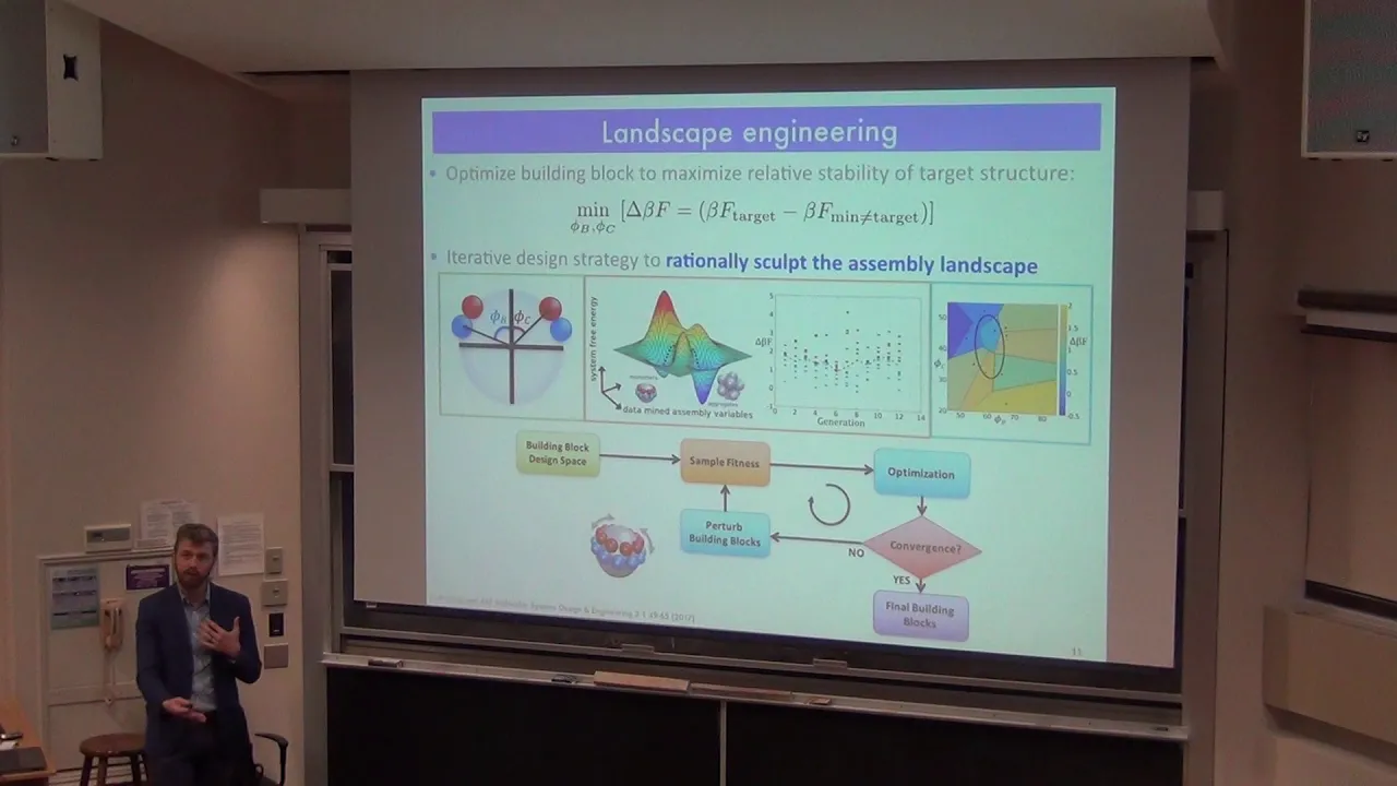
pathways connecting them okay so that's how we recover the landscapes how do we then do the second part which is to say okay I have a landscape corresponding to one particular building block how should I change the properties off my building block to make that landscape more like I want it to be I should stabilize the structures the self assemble materials that I care about so we're gonna use genetic algorithms to do this And so given these landscapes this provides us a powerful way to do the inverse design because we can ask the landscape to

sort of change its morphology to sort of stabilize perhaps you want to stabilize this structures to make this free energy well really deep destabilize this structure because it's going to push the system away from this and push it into this this free energy minimum so you can define a number of objective functions over this landscape The simplest of which perhaps is the following you want to sort of maximize the distance between the free energy of your target structure and the free energy of its next competitor so that's to say let's find the the free energy

of the wild that we care about our target free energy well let's find the free energy of its nearest competitor and let's make that gap as large as possible and so that's going to stabilize the Thing that we want destabilize the things that we don't want you can think of more complex objective functions may be minimum action pathways fancier things but this one is a pretty generic one that there works quite well and although it's a purely thermodynamic metric because you're actually changing the overall global topography of your manifold it actually also effects the kinetics

which I will show you also okay so so given our objective function and How do we run our genetic algorithm so we pick a bunch of initial candidates so these are patchy colloids so this is so I'm going to tell you about which are basically sort of micron sized colloids with sticky patches on them and so these sticky patches are specific and so the red sticks to riding blue sticks to blue and you can think about this as sort of being functionalized with DLA DNA all that goes if you wish and so these are specific

interactions between these These sticky patches okay so you see you pick a bunch of these you think might be reasonable candidates you find they're assembly landscapes and you measure the objective function for each one of those candidates so this is generation one here's the fitness of each one of these candidates according to our metric Delta beta F which is this gap and then you say okay who are the good guys who are the bad guys make the genetic algorithm move us more towards the good ones and So here's our design space where in this case

it's 5e and Phi C which is just the angles of these things so find the ones that are good use those to seed the next generation of candidates through this genetic sort of crossover algorithm where you apply mutations and crossbreeding to seed your next generation so here's generation 2 and then you just move along this generations until you converge and so basically you can think about this in The following flow diagram you have some initial building blocks they may not be particularly good ones you can sample their fitness landscapes you can run the genetic algorithm

ask if you converged and so if you've not converge die you've not sort of reached some global optimum Yury perturb your building blocks through this G a and just keep moving around this loop until until you reach convergence and that will give you your final building blocks so basically what We're asking the the machine learning or the genetic algorithm to do is change the building block design in a principled manner to make the landscape look more like we wanted to to stabilize the materials that we care about with the structure or the function that we

want okay so let me give you an example of this so we've used this to assemble sort of polyhedra and two structures that we care about so things like icosahedra Encapsulants looked like viral capsids or perhaps octahedral clusters all of the Platonic solids very recently we've actually applied this to infinite aggregates ie crystals and so so why NARTH would you want to make a colloidal crystal so cláudio crystals turn out to have this this beautiful property that they're just of the right land scale and if you can make them assemble particular crystal morphologies with open

architectures they possess Omnidirectional band gaps at visible frequencies so it's a why is this valuable well it turns out that photonic crystals are two photons what semiconductors are two electrons and so if you can design photonic crystals with omnidirectional band gaps meaning three-dimensional band gaps in visible frequencies you can use them as sort of wave guides for light and this is an enabling technology for sort of optical computing and so there's a lot of Interest in synthesizing these things so what's the problem with these so it turns out that we possess one in 2d photonic

crystals we know how to make these pretty well 3d photonic crystals are challenging why because the 3d photonic crystal architectures are very open architectures with very low atomic packing fractions so these things do not occur naturally they're just to open lattices to sort of generate using simple sort of hard spheres or sticky Spheres so you really need directional interactions to synthesize these things and it's very unclear how to have robust directional interactions that will make these with high fidelity so here's a couple of examples of photonic crystals the the canonical diamond lattice and it's inverse

in which case if you put tetrahedra within all the gaps of the diamond lattice you wind up with the pyrochlore lattice this is what I'm going to be talking about today so turns Out this pyrochlore lattice has this bandgap at optical frequencies and it turns out you don't need a very large or refractive index difference sort of a dielectric contrast between your colloids and your matrix which is typically air so it turns out even with with just 3.14 3.41 which is for silicon or maybe a little bit larger for other materials you can open up

a bandgap very easily so these are nice systems that have desirable properties the question Is how do you assemble them so can we use our inverse design procedure to tell us how do we place directional interactions on these fears in order to assemble these open lattices okay so if we look at the pyrochlore lattice it turns out the fundamental motif is a stacker staggered tetrahedron and so if you look at a particular particle and you look above you will see that it has three neighbors in this sort of triangular configuration so this guy Forms a

tetrahedron if you look below it it also has these three neighbors in this tetrahedral configuration but this type this set of three is staggered from this set of three and so they're sort of moved by sixty degrees and this is a fundamental motif you need to assemble the pyrochlore lattice you need the guys above you to be staggered by sixty degrees from the guys below you so how do you form how do you design particles that will have that behavior well the Simplest way to do this is to assign each particle three sticky patches on

its North Pole on its South Pole that are staggered by 30 degrees so here's a North Pole here your blue sticky pad cheese this gray sphere is translucent so you can see through it here's your South Pole with these three sticky patches so that will give rise to this architecture so the question is where should you place these patches and how sticky should they be in order to Assemble the pyrochlore lattice and so it turns out they should not actually be directly on what you would believe should be the Platonic ideal locations you need a

little bit plasticity there to account for entropic effects and you also need to worry about healing defects in your pyrochlore lattice so if you just design these patches and run the assembly you typically end up with mass and so the way to actually get this is a little more subtle okay so here's the Idea we use our inverse design to sort of engineer a two-stage hierarchical assembly procedure so what do we do okay so the patches are gonna look like they're sort of a sticky patch on the North Pole there's a sticky patch on the

South Pole we're gonna make the North Pole a little more sticky than the South Pole so why we do we want to do that so it allows us to do a high temperature assembly where the sticky north poles form these tetrahedra and then it allows Us to do a low temperature assembly where the South Poles then become thermally active and they cos can assemble the opposing tetrahedra the staggered tetrahedra so this thermally decouples these two things and allows us to make a mono dispersed mixture of tetrahedra that are subsequently assemble into our pyrochlore lattice and

this is not a new idea it's sort of a two-stage Assembly hierarchy and to make sure we don't incorporate too many Defects and so it allows us to make these things perfectly in the first stage and then assemble them very slowly under a temperature ramp so the particles have enough energy he'll defect to make our pyrochlore lattice okay so how should we engage this this this design problem so okay so this is just I wanting to point out so here's an example of this staggered tetrahedron so if you look at this middle particle here upstairs

you have This trying over where this pointing sort of towards you downstairs you have this triangle is pointing away from you so this is a fundamental motif we're gonna ask our landscape engineering architecture to sort of figure out for us by stabilizing the tetrahedral motif okay so here's an example of this office optimization procedure so we did exactly what I described we we find our landscapes we run this inverse design procedure and we run it for a number of Generations until we converge so what am i showing you here so I'm showing you two different

spaces so up here is our optimization space what are we optimizing we're optimizing the angle and the strength of the interaction of the North Pole so if I go back one we're optimizing the angle and the strength of the interaction of the patches on the North Pole's basically where do we place these patches and how stick you should they be so we're just worrying about one Pole right now because we just want to make this high temperature assembly so how do we stabilize this guy to form tetrahedra at this high temperature okay so we start

with an initial set of candidates the black dots are our candidates and so they're dispersed all over this design space so different degrees of stickiness different angles at which we're placing these patches are all over the place and here's our objective function the stability of the Target structure this tetrahedron relative to its nearest competitor so these things are typically green and yellow which is relatively high so it's a bad value of this fitness function we want to push things towards blue what am i showing you down here this is an example off the assembly landscape

for the fittest candidate in that generation so these guys are the eigenvectors that came out of the diffusion map these are collective variables in which we build Our free energy landscape and I'm showing you the free energy landscape and so here's our monomers they have a particular free energy here's our dimers they have a particular free energy trimers tetramers and pensa Murs so it turns out the tetramers are not the global free energy minimums it's a relatively bad initial design but that's okay we asked the genetic algorithm say what are the best guys from this

generation Let's seed them use them to seed the next generation and repeat this procedure so by generation 5 things have got a little better so you can see that the distribution of candidates is now a little bit tighter so this this oval is just showing the two principal axes of this distribution it's starting to tighten up it's starting to move towards this region of space things are a little bluer so things are a little fitter and here's The free energy landscape for the fittest candidate in this generation these eigenvectors are totally distinct from these ones

because it was it was designed for a new generation so the diffusion map operates only within a single generation and now we can see that the tetrahedra a little more stable relative to all of the competing oligomers this is this is an improved design okay by generation 15 we converge so how do we decide we converge well Basically we're within 1 kt with an energy space and within 1 degree within the patch angle so this is our criterion for convergence the distribution is now very tight the fittest candidate from this generation is sort of moved

towards this this very tightly distributed region of space here in our design space and you can see the the tetramers are now overwhelmingly the most stable configuration who've actually completely destabilized the trimers dimers and Monomers within the resolution of our sampling and the only competitor of these pan tumors which are much less stable than these tetra MERS so the inverse design procedure has told us exactly how we should make the patchi's placed and sticky to favor in the assemble of tetrahedra over all competing aggregates ok so here's the the optimization time course so starting from

generation 1 we at our initial guess we have high variance in this Initial guess because we had many many candidates and as you run through to generation 15 this thing oscillates for a while and then converges to around 15 point 5 degrees and so this is where you should place your patchi's excuse me 15 point 5 kt and so that's how sticky you should make your pad cheese 5 years is the patch placement and so it turns out you should put them at about thirty point five degrees which is not exactly where you should anticipate

you would Put them just based on geometric constraints and so the optimizer also accounts for the the entropic entropic forces in this optimization because of course is a free energy not just a potential energy and so that's baked into the way that we place our pad cheese okay so this told us that in order to assemble tetrahedra at this high temperature which is a reduced temperature of 0.8 this is how you sticky you should make the guys and this Is the angle at which you should place them so that's good and so we can run

high temperature assembly and make tetra deidre with high fidelity so we've stabilized the formation of these tetrahedra but I said I want to also do the second stage of the hierarchical assembly and unform pyrochlore lattice from these tetrahedral building blocks so how do we convince our our inverse design procedure to do that for us so it turns out we actually don't need to do Anything new we can just sort of extrapolate the results for the North Pole to the South Pole because all we want to do is also make tetrahedra but it turns out all

we want to do is make them in a staggered orientation so you just move your patches round by sixty degrees without changing the angle Phi B so here they're still at thirty point five degrees or just rotate you run the azimuthal angle by sixty degrees and how sticky you should make them well you Just extrapolate to the low-temperature which you want to form your assemblies and so instead of being at point eight you're at point three so you just rescale the stickiness of your interactions accordingly and so actually we don't need to run a new

round of inverse design we just use our high temperature results and extrapolate to low temperature okay so the idea is we've stabilized this intermediate motif and then we believe that we can then use That as a building blocks to assemble the final pyrochlore lattice okay so does this work so let me show you first of all the high temperature assemblies this is stage one of assembly here's the initially monodisperse distribution of these these patchy particles with the design that the inverse design algorithm told us to use and then we run our brining dynamic simulations actually

is Langevin dynamics and we see that we assemble mono dispersed tetrahedra so This actually worked very very well so here's the pair correlation function of the tetrahedral centers and in the terminal frame so you can see that basically you have a small peak here but basically you're an ideal gas of tetrahedra and so there's very little structure so this is good is telling us the North Pole's are causing these guys to assemble a high temperature but the South Poles because they're thermally decoupled they're very unsticky at this High temperature are not causing these things to

aggregate and make sort of messes with with imperfections it's really just a mono dispersed mixture of tetrahedra so then we use this simulation and then we apply a temperature ramp so now we're going to slowly ramp the temperature from our high temperature and reduce units of 0.8 down to 0.3 so we do this over the course of five times ten to the eighth steps and this is a very slow ramping Which gives the system plenty of time to sort of rearrange and heal defects so here's this temperature ramp where we ramp down into this low

temperature and so we start with our monodisperse tetrahedra these guys move around in space and then eventually you'll see the back of the box this pyrochlore lattice is going to nucleate and then all the system is going to collapse into this near-perfect pyro Lori pyrochlore lattice so in the the movies going to Circulate ryan and so you can see that this is the pyrochlore down here we actually have a grain boundary up here so you'll see these guys are dimers not tetramers so the thing is not a perfect lattice but down here it's a very

high fidelity pyrochlore lattice and so we checked that by looking at the pair correlation function and so these delta functions in orange are the peaks of the ideal pyrochlore lattice and blue are the results from our last frame of our Simulation so all the peaks are in exactly the right places and here we have the the q4 parameter which is a Steinhardt bond order parameter of the fourth order and so if we were an ideal pyrochlore lattice this should be centered around 0.02 and it is and so our Gaussian distribution lies there this little shoulder

here is essentially just finite size effect since it's because we don't have an infinite lattice we have sort of edges to our Pirate Laurence's so we understand where this is coming from and so this inverse design procedure has told us how to design a building block to stabilize the formation of this photonic crystal and so we think this is a nice interesting result it provides a prescription to sort of design and interactions on this colloidal building block to assemble this useful photonic crystal and so we're taking this now to in a couple different directions and

so we like to Design also the diamond lattice which means that we'd like to design a tetra Mar and and a dimer end and so now what we will to assemble Dimond if we're able to do that and also check the robustness of this so this is a mono dispersed design and so all of our designs have exactly 15.5 katie's of stickiness and 30.5 degrees of angle of course when you're making these things experimental you're gonna have some poly dispersity so how robust are we to poly dispersity Is gonna be a really important thing to

try and engage here okay but those are easy things to bake into our design protocol you just apply some dispersity to to your to your genetic algorithm ok so with that I'd like to sort of move on to the second story which is also using some machine learning techniques but but a completely different machine learning techniques to try and accelerate molecular simulations okay so this is what are we doing in This space so the idea here is that it really goes back to this idea of Martin Karr places' 1990 paper with a Greg pets code

and like a dynamic simulations we basically suffer from two limitations so there are systemic errors due to the the potential energy functions ie the force fields and there are statistical errors due to sampling and so this means that our force fields are not perfect that introduces some systematic errors and you have to run your simulation long Enough to get converged thermodynamic averages and all as you run for the age of the universe you're not going to make sure that your converged and so we have sort of configurational sampling problems and so this paper from 1990

is equally true today we're still grappling with both of these issues and so what I'd like to tell you about today is some ways that we're trying to think about improving the second one so how do we do a better job of sampling configurational Space with the finite computational resources that we have so this is an old problem and so we know a number of ways of doing this so we can use accelerated sampling we don't just run unbiased molecular dynamics that evolve according to Newton's equations of motion we perturb the equations of motion to

allow us to do a better job of sampling space we push the system around it's its phase space to try and do a better job of sampling and a better job of getting Converged thermodynamic averages so there are basically two classes of ways of doing that tempering techniques which seek to modify the temperature or the Hamiltonian of your system in order to improve sampling so basically you want to modify the Hamiltonian such your energy barriers are lower and you can push the system around more easily the other way of doing things is to sort of

leave the Hamiltonian intact but shove The system around with some artificial biasing forces so you push it around with some artificial potentials that help you move through the phase space and do a better job of sampling and so these are basically collective variable biasing Taney's you need to define some good collective variables in which you sort of accelerate your system and there are a number of ways of doing this the oldest one is sort of perhaps umbrella sampling there are various fancier Flavors of this so method dynamics which is one that professor Widmer works on

a lot but the big question with this is how do you define good collective variables in which to design your sampling algorithms and so how do you find good directions in which to apply your artificial biasing forces if you pick bad collected variables then you do a terrible job and yours wasting a bunch of computation and for all that the simplest Systems it's very hard to intuit what is a good collective variable and so can machine learning help tell us what good collective variables are and then uses collective variables to apply biasing potentials and do

a better job of sampling configurational space okay so there are many ways of finding collective variables and so what sort of properties should they have and so good collective variables should separate out the metastable states of the systems you Want to do a good job of doing that they should characterize the the slow configuration of motion so they should characterize the dynamics of the system and so so far what I've told you diffusion Maps seems to be a good candidate and so what I showed you in the previous part of the talk was the diffusion

maps are very good at doing that where did diffusion Maps fall down they're not explicit differentiable Functions of your input coordinates that's to say if I run a diffusion map on your molecular system I can get some low dimensional embedding but I don't know how to write down an explicit expression taking the atomic coordinates to your collective variable space why is that a big deal well you need that explicit expression to propagate biases to the atomic to the two atomic forces so if you write down a biasing potential within your collective variables to Shove the

system along these collective variables you need to propagate that force back to the the atoms in your system to run your molecular dynamics simulation so if you don't have that explicit differentiable mapping you can't do that okay so I really need that in order to be useful so okay well one class of methods it does have that explicit mapping or linear dimensionality reduction technique so principal components analysis Multi-dimensional scaling they do have that explicit mapping in that respect they're very good however they don't do such a good job in the first two criteria nonlinear dimensionality

reduction techniques such as diffusion maps ISO map look locally linear embedding again they do well on the first two they fall down on the third so what is the technique that allows us to hit all three of these criteria simultaneously so it turns out that deep Neural networks are actually this is a shallowest variant of deep neural networks but Auto encoding neural networks are one way of doing this they allow you to hit all three of these criteria and provide a useful way of finding good collective variables that you can then do direct do enhance

sampling directly within those variables okay so so to my knowledge it's one of the only or invite the only nonlinear dimensionality reduction technique that Gives you this explicit differential mapping between your collective variables and your input coordinates in this case atomic coordinates so it's very fashionable deep learning is sort of a nice technique to use in many places this is the reason we're using it and we believe that it's one of the most powerful methods we can use to engage this problem okay so how do we use this the particular flavor of deep neural networks

we're using our auto encoding Networks or so-called also encoders so what are these it's an unsupervised machine learning technique so what are we passing to the input layer we're passing atomic configurations we've done a little molecular simulation we know what the molecule looks like we have its Cartesian coordinates as a function of time and we ask the neural network can you find good low dimensional collective variables with which to describe the dynamics of the system so how do we do That well we design a neural network architecture with this Auto encoding topology so here's your

input coordinates here's your so-called hidden layer that's actually doing the computation your encoding and here's your bottleneck layer so here's the low dimensional latent space you're trying to learn so okay if you were if you knew the collective variables a priori you could just train the encoder to do that but of Course that's a problem we're trying to solve we don't know what these collective variables are so how can we discover them well you strap on a decoder this says take these collective variables and try and reconstruct your atomic coordinates that you started with so

the input and the output and the ideal case should be the same so what are you asking the network to do you're saying can you take my high dimensional atomic coordinate discover a low Dimensional representation from which I can reconstruct my atomic coordinates with high fidelity if you can train the network to do this you know you've discovered a good low dimensional representation and this low dimensional representation is exactly the collective variables that we want to use to do our sampling because it tells you you can preserve most of the dynamical information about the system

in this low dimensional latent space okay so that's Good and why is it explicit in the differentiable well neural network is nothing more than a bunch of sort of weighted sums of inputs passed from one layer to the next sort of modulated with some nonlinear activation functions so all of this math is explicit so I can write down an explicit mathematical expression relating this collective variables to the input atomic coordinates and guess what the way you train your rule network is by gradient Descent back propagation so you have the gradients for free so you have

your biasing forces automatically okay so unsupervised learning trying to find a low dimensional latent space representation that's explicit and differentiable okay so here we're actually specializing to molecular simulations so here you have some configurations of your molecular system the N coding layer is taking through you from your high dimensional Space to your low dimensional representation you're decoding layer is taking you from your low dimensional representation back to your high dimensional space so we perform training using the encoder and the decoder once you've trained your network and you find your latent space representation you can throw

away the decoder you don't need that anymore all you need is the N code or the mathematical transformation that goes from the input to the to the Bottleneck layer so how do we train these things and so we just use standard back propagation algorithm and so basically we're trying to minimize the reconstruction error subject to some regularization so here we have the reconstruction error and so this is your input coordinates of your atomic system here's your reconstructed coordinates and some more explicitly you run your input configuration through the N coder back through the decoder see

how well Your approximate your input take the l2 norm that's your reconstruction error would also like to stabilize fitting by applying a regularization term so this is just the so-called weight decay so this is just providing sort of a penalty on having very large weights in your network which is basically just the parameters of the network you're trying to regularize those towards small values to improve the robustness of your fitting how do we fit this we actually Use sort of a variant of cross-validation so it's a little bit fancier than that but basically we just

split our dataset into training and testing sets and we terminate training when the testing errors reaches its minimum okay so that's how we train our network and so we collect a small amount of molecular simulation data we train our network that gives us an initial guess for our collective variables how do we specify the dimensionality of the System so a priori we don't know what the dimensionality is going to be and so we know it's going to be something relatively low so for all molecular simulations molecular systems that I've ever studied the dimensionality is always

been between around 2 and 7 so it just seems that natural proteins are arranged to be low dimensional perhaps you can speculate that in order to do some evolutionary useful work you need to populate a low dimensional manifold But empirical data suggests you're relatively low dimensional but we don't know how a low dimensional so how do we figure that out so we do that again by cross-validation and so we train a bunch of all two encoders with different numbers of bottleneck nodes and so this is a two-dimensional latent space if you have a third node

here that's a three dimensional latent space we train two three four five six seven and we ask how does the fidelity of your Reconstruction and the output layer depend on the dimensionality of your bottleneck layer so this curve here is basically showing the fraction of variants explained as a function of the number of nodes in your bottle night layer so if you only have one node you get about 70% if you have two nodes you have about 80% if you have three nodes you have about 90% and then you asymptote so in this case we

would say up right about three nodes is the right To mind that's the knee in this curve so we probably have a three-dimensional latent space so this is a systematic way of analyzing the data to tell you your intrinsic dimensionality okay all right so then we train our network it seems to go pretty well so then how do we actually implement the bias and so here we apply our bias generically through it's or an artificial potential so here's the probability of particular molecular configuration so the Boltzmann Distribution is is to be the distribution that we

care about so here our this is the energy of the system and so the energy is composed of sort of your unbiased Hamiltonian so that's the natural force field for your system this is whatever amber or charm or gru max tells you the force field is and here's our artificial potential so we write down our artificial potential this biasing potential V as a function of our collective variables which themselves Are a function of the atomic coordinates so these CBS are explicit and differentiable functions of the atomic coordinates that's why we used also encoders in the

beginning so if you're running Monte Carlo simulations you can write down the energy as a function of the unbiased Hamiltonian and the biasing potential if you're running molecular dynamic simulations you can take first derivatives and write down your forces as a function of unbiased forces that Come out of your molecular simulation engine and your biasing four-season you can explicitly write down as a function of your collective variables so this is how we're pushing our simulation around the collective variable space in collective variables that we've discerned directly from the data so a vasa system to tell

is good collective variables and then we exploit those collective variables to enhance sampling okay so this is good so what's The problems the problem is you have a bit of a chicken and an egg problem you need good sampling of your configurational phase phase to get good collective variables but you need good collective variables to get good sampling of your configurational phase space so what do you do and so you use some sort of bootstrap iterative technique and so the idea is you sort of interleave simulation and biasing so you do a short unbiased simulation

you don't Do a very good job of populating your phase space but you learn some reasonable collective variables with which to drive your system using these biasing potentials you drive your system you do a bit that's your job of populating the space you then learn even better variables you driving those variables etc etc until you converge this idea of sort of interleaving sampling and learning is sort of the the sort of the sort of iterative paradigm That we're gonna exploit so online biasing using the the learned collective variables offline learning to learn better collective variables

each time so this might look something like this block diagram so in iteration zero maybe you run an unbiased molecular dynamic simulation you train and also encoder to learn some variables you do some biasing those variables you expand your face based search you then perform some umbrella sampling here to expand out Your regime of sampling learn new phase space variables so you're pushing out to a larger portion of space larger and larger and then you terminate when you stop when you get diminishing returns basically when your collective variables stabilize and you stop enlarging your sample

region of phase space okay so let me I describe for you a couple of examples and just gonna talk about the first one and the third one so the first one is alanine dipeptides is sort of the Hydrogen atom of protein folding super simple system we understand it very very well let's use this as a test case for our algorithm okay so here we are so we did exactly what I described and since let me show you the real data for this and so the last step flow diagram I showed you is just a block

diagram here's the actual data okay so what am i showing you so the first column is basically the collective variables learned by our auto encoder C 1 and C 2 as a function of three different iterations this is iteration 1 3 and 5 so here we're projecting the data that we get from an initial unbiased simulation of our molecule into these two collective variables the first autoencoders is learned I'm coloring these by the Phi angle of the the backbone to heed rule so it turns out dial mean it's not terribly important as well described by

the phi inside backbone dahi drills we know those are Good collective variables so can they also include or learn that and use those to accelerate sampling so here we've colored the data by the Phi angle here is exactly the same plot where the data has been colored by the Sai angle and here's a Ramachandran plot where I'm just projecting the data from this initial unbiased simulation into Phi size space so we're restricted to sample this upper left corner of the diagram would really like to sample this whole Surface okay the blue crosses are for we

initialize our first run to BI simulations this is where we say okay these are anchor points where we would like to apply harmonic biasing potentials to push the simulation out sample these new points so we're trying to expand the region over which we do our sampling so by iteration three you have been reasonably successful we've pushed out this region of sampling out a little bit further this is populating a Larger region of our collective variable space you can even see in the Ramachandran plot when I sort of populate through this entire left column so so

things seem to be going reasonably well but as you'll see between iteration 1 3 and 5 things are changing all the time these collective variables are not the same between each iterations who have not yet converged and certainly the region of sampled space is changing telling us we've not done a good job of Fully sampling the phase space iteration 7 is the same but then between iteration 9 and iteration 10 we see actually some convergence so it turns out that the collective variables discovered an iteration 9 and iteration 10 are identical up to a sine

flip and so it turns out if you just flip the signs of this this manifold here you get this manifold right here so you flip it this way flip it this way you can even see that these things look the same so our Collective variables have stabilized also the region of the manifold that we populate even though we try and bias to push it out further it doesn't go any further we sort of reached the limits of thermal sampling and so we've sampled the phase space sort of comprehensively and so we should believe that we

should get some nice converged averages so you can also see this in the Ramachandran plot and so you can see that there's no expansion and training between the Saturation and this iteration so we sort of say that we've done a good job of sampling and then we find our free energy landscape and it turns out this free energy landscape is in quantitative agreement with the one that you would have gotten if you just run unbiased simulations for a very long period of time so because we can do that for the alanine we know the gold

standard answer and we can verify with our technique actually got the right answer okay so so Why should you care what's the advantage well the fact is we can do it very very quickly without knowing any a priori information about the system so this algorithm I just described figured out what the important collective variables were figured out what the dimensionality of the system was figured out how to do by a sampling in that space and that it all very very rapidly within 22 CPU minutes whereas this is required orders of magnitude longer simulation to do

This using biasing techniques excuse me using unbiased techniques okay so then you might say well why don't I just use meta dynamics or my favorite by simulation technique in this case you could do that because you know they collected variables but our methodology was able to discover the collective variables for you so for assistance when you don't have that prior knowledge this is a great value okay so that was for on for a leading dipeptide so a super super Simple example so what about something a little fancier so we think this is a little fancier

you may not agree but the reason it's a little fancier is because we're trying to directly engage solvent coordinates this is some work that we're doing with Hamish Patel at University of Pennsylvania and the problem is of following a lot of protein folding really depends very heavily on what the solvent is doing you can't just focus directly on what the protein atoms are Doing hydrophobic effect is the main drivers of protein structure and function okay so we know that so that tells us that when we're doing these learning techniques we should really be engaging solvent

coordinates directly so we said okay protein folding is difficult we'll build up to that let's start with something simple let's start with a hydrophobic polymer chain and ask if we can use these Auto encoding neural networks to tell us well what are the Important solvent variables we should worry about and how should we buy us on the solvent coordinates to help us understand how the system is folding and ultimately how we can then accelerate sampling okay so this is an example of the folding of a polymer chains is just simple c24 alkane is living in

water this bubble around this is just the solvent excluded volume and so you can see it starts to fold up it makes this kink in its head the solvent bubble Grows to encompass the entire chain the sort of solving excluded volume stabilizes this collapse configuration you'll see in a moment the solvent bubble then breaks and the sort of a molecule then extends back out to to an extended state so we know that solvent is really really important in understanding the dynamics and the thermodynamics of this system so can we sort of engage that question using

all two encoders Okay so so let's step back for a second and say well what about if you don't care about the solvent let's just learn over the solute coordinates so let's learn over it exactly what we did before for die alanine just worry about the carbon atom coordinates of this polymer chain so you can do that I explained to you exactly how we do that so here's our autoencoder here's our atomic coordinates here's our reconstructed atomic coordinates here's our latent Space and we learn this latent space representation that we can then use for biasing

okay so it turns out this guy is two dimensional so the fraction of variance explained curve tells us we're two dimensional here's our first variable here's our second variable here's the embedding of our data point since this low dimensional space and I've colored them according to the first principal moment of the gyration tensor which is just telling you how long the Chain is so here we have the all-trans chain here we have the helical e collapse chain it's living in a solvent bubble and here we have some intermediate configuration and while we note from this

plot is there's this big hole in the middle so what is this so it tells us that as this chain is collapsing it's not collapsing like this it's collapsing like I showed you in the movie by making a kink and either the head or the tail and the chain then Slides down and collapses so why is it doing that it turns out that in order to collapse like this requires a collective expulsion of solvent molecules that's free energetically very costly it's much cheaper from a thermodynamic perspective to push the right one by one and so

the auto encoder is able to learn that it tells us that this is the collapse pathway to go around the outside okay so what about the second variables the second variable c2 that was discovered By the auto encoder so this guy right here is well correlated with the vertical shift of the ends of the chain so it tells you whether you have a kink in the head or whether you have a kink in the tail okay so these are good variables with which to describe the system good variables with which to accelerate the systems you

could accelerate along this first mode or along the second mode and things go and things go reasonably well these are good Solute acceleration variables all right so I said the purpose of this was to try and engage the solvent so how do we do that so let's pretend we don't know anything about the solute we don't have the solute coordinate so we can engage is a solvent can we learn something about dynamics of the system and how well how far does that get us to describing the chain collapse dynamics so I just want to do

this so maybe you just plug into your author encoder the Coordinates of all of the solvent molecules so it turns out that's a terrible idea so because they're an solvent molecules and they're all identical and so you have this n factorial relabeling problem so all real labelings of your solvent molecules do not change the state of your system there's a symmetry that you need to engage so we don't want the auto encoder just to learn that solvent Molecule one should be over here and so on molecule twelve should be over here whereas if you exchange

them this is a state of the system doesn't change so you need to do something that mods out that symmetry so what do we do so we use some tricks taught to us by it by Amish Patel which says well let's draw a little spherical volume around each one of these solute atoms and current how many solvent molecules live inside there so we actually use a smooth count so we Don't get any discontinuities from sort of solvent molecules passing over this boundary but basically it's a it's a smooth number of counts of solvent molecules in

the vicinity of each solute atom how big do we set the volume of the sphere well basically we pick the sort of first trough in the pair correlation function so this is where the solvent molecules are sort of moving in and out of the hydration shell okay so then we can the solvent molecules inside each One of these little spheres and we passed that to our autumn encoder we then asked the auto encoder to reconstruct these solvent cans this is a pure solvent off to an encoder okay so what happens and so we learn the

following collective variables so these Zeta 1 and Zeta 2 or the solvent collective variables we can project our data into the solvent collective coordinates and how do things look so it turns out we get very similar manifolds Its first of all it's two-dimensional and the the two dimensions that we get are very close to the ones that we got from the solute collective coordinates so this first one here is a 2 one is basically correlated with the some of the solvent counts and so the Sigma is just a sum of the number of solvent molecules

and all of these spherical volumes and so this guy is basically you can think about as being wet and this is a elongated configuration where all the Solute molecules can get very close to the chain this guy here is very dry why is it drive because hydrophobic lis collapsed and so the auto encoder learned this is a first important mode basically how wet or dry the chain is while ray the second mode the Zeta 2 so this basically corresponds again to this Delta and so this is how a kink the chain is where there's a

kink at the head or a kink in the tail but of course the alter encoder doesn't know anything About kinks and the solute so how does it represent that it basically represents them as basically whether the head is dry or the tail is dry so in this case the hi is gonna be wet and the tail is going to be dry and in this case the head is going to be dry and the tail is going to be wet and so basically learned whether the kink is in the head or the tail ie the hydrophobic

collapse has occurred at the head or the tail of the molecule so Basically we get I'm not sure whether it's quite by ejected but we get similar information content about the folding process from the solvent coordinates moreover we can then bias directly in the solvent coordinates and ask if we can accelerate our sampling so here we go I'm biasing in the first coordinates a21 and so when we bias a 2-1 to be towards the left hand side of the diagram things are pretty wet and so I've not pushed out much of the solvent Molecules as

you apply stronger and stronger biasing potentials you're causing dewetting of the solvent away from your chain so what is this doing it's basically building a solvent bubble around your chain and by doing that you enhance sampling so here we restricted to the very elongated chains that are very wet by the time we get over here we're sort of oscillating freely between elongating and collapse chains why because I basically remove the chain to The ideal-gas and so now there are no solvent molecules around to sort of prevent collapse or extension happening and the chain is very

happily sampling in and out of the collapse configurations this is a different way of accelerating the system by modulating the solvent coordinates okay so hi by device sample not in the horizontal direction but in the vertical direction so can I make the chain kink in the head in the tail and the answer is yes and so If I move towards sort of the bottom of the diagram I can make the head dry by pushing the solvent molecules out and keep the tail wet if I push up to the top of the diagram I can do

the inverse and this induces chain collapse by either one of those pathways head kinking or tail kinking okay so both of these are ways of accelerating your dynamics using the solvent alone so this is just proof of principle it's sort of a relatively simplistic example and of Course we would like to combine both the solvent and the solute because coupling between these things is likely to be very important in sort of real proteins when these things are not happening in isolation you have solute and solvent talking to one another and we like to apply it

obviously to more interesting systems than a simple hydrophobic polymers so systems that are very difficult to sample perhaps proteins with bound water molecules for biasing On the protein alone is not going to get you a good sampling you need to also bias on the salt and okay so all of this stuff is freely available on github and so so my students sort of implemented all this as plugins to open mmm and we're also working with the developers of bloom add the enhance sampling suite to sort of baked this into the the flume at libraries and

so it should be very easy to sort of I use these techniques within Your own molecular simulations if this is something you're tall care abide and so ongoing work so the first part of the talk and so we're like I said we're doing universe design if the diamond lattice everything I told you today was engineering colloidal level systems would also like to engineer sort of molecular level systems so how do you design a peptide that particular self-assembly properties to make sort of elongates it sort of by electronics that Are sort of biocompatible and ultimately sort

of a complementing our computation with some experimental synthesis and so can we actually use this engine to try and direct experimental synthesis towards promising designs second part of the talk again like I mentioned coupled solute solvent extraction applying it is sort of more interesting proteins of allosteric transitions and large proteins where a sampling is very difficult and we think this methodology Can really ameliorate the difficulty and sort of reduce the amount of computational effort one needs to go to and then using these latent space representations to design generalized lanzhou on equations or multi mark off

state models to try and improve sampling by sort of running the dynamics within the latent space and then projecting back up to your high dimensional atomic space okay so with that I'd just like to I think the funding sources and so this Has been largely supported by NSF and Department of Energy and the folks that did the work and so in the first part of the talk and the landscape engineering that was Andy long he's now a data scientist at 3m Utama who's with me in Chicago and the second part of the walk work was

done by my my student HN and so with that I'd like to thank you for your attention and take any questions that you might have yeah I mean it's good question so if You're if you do have disjoint regions and your variance in the design of your candidates is not sufficiently broad then you will have difficulty finding that for sure so I guess we're appealing to concepts of sort of smoothness and locality and so in the design variables we've picked so far those are smooth continuous variables in this case it was a stickiness to an

energy and it was an angle of the patch it becomes way more Difficult if you're in a discontinuous space so I'm thinking sort of molecular space or you're sort of design variable is a smile string or something like this in that case I think you have big concerns about your ear disconnect ippity yeah I think it's a great point so the algorithm that we use is pretty robust for these relatively smooth spaces I think we use covariance matrix adaptation yes a lotion strategy for disconnected spaces I think other things May be more appropriate we think

it's okay for this yeah but I think you know things are like a lonnis part of guzik worries about here here's some fancier algorithms that for chemical space that I think we could appeal to so when you talked about using an assault that counts in order to get rid of the permutation difficulty that implies to me that you can't go back and generate a configuration yes that's a great point Sure so the question was when you solvent counts run the solvent coordinates does that mean that you no longer can represent rigorously the the high dimensional

state of the system I'm answers yes and since that's absolutely true so what you then have is a statistical dependence there are multiple realizations of your high dimensional system they're consistent with your low dimensional embedding if you like so I guess the way you can Think about or at least the way that I find useful to think about it is that we've sort of added an extra layer here if you like that we've gone from our atomic configuration and sort of by Fiat we would sort of coarse-grained that in two currents and that's what we

passed the neural network and the neural network doesn't know anything about the configurational space anymore and so they're multiple realizations are consistent with that but that's okay Because the solvent configurations are consistent with your low dimensional projection or the ones that you care about and so if you care about this in a statistical sense rather than a by active sentence I think that's okay so if you are really worried about okay I think that the positions of the molecules and exactly how far they are from the the solute atoms rather rather than just their coarse-grained

counts are important then you would have to do Something coordinate based and there's work by y9e at Princeton who used similar can similarly descriptions to them so they actually use a very nice trick which is that I talked about a fungibility problem this n factorial relabeling all they do is look out to a certain distance and order the solvent molecules according to distance and so the first molecule you present your autoencoder is a closest one the next one is the next closest one and so you Always have the correct ordering at least in distance space

in the way that you present them and that seems to work reasonably well well thank you very much come here Thanks [Applause]