CS 285: Lecture 5, Part 3

so in the next portion of today's lecture we're going to talk about how we can modify the policy gradient uh calculation to reduce its variance and in this way actually obtain a version of the policy gradient that can be used as a practical reinforcement learning algorithm the first trick that we'll start with is going to exploit a property that is always true in our universe which is causality causality says that the policy at time t prime can't affect the reward at another time step t if t is less than t prime this is another way

of saying that what you do now is not going to change the reward that you've got in the past now it's important to note here that this is not the same as the markov property the markov property says that the state in the future is independent of the state in the past given the present the markov property is sometimes true sometimes not true depending on your particular temporal process causality is always true causality just says that rewards in the past are independent of decisions in the present so this is not really an assumption this is

always true for any process where time flows forward the only way this would not be true is if you had time travel and you could take an action or travel back into the past and change your action but we're not allowed to do that all right so i'm going to claim that the policy gradient that i've derived so far does not actually make use of this assumption and that it can be modified to utilize this assumption and thereby reduce variance you can take a moment to think about where this assumption might be introduced the way

that we're going to see this is we're going to rewrite the policy grading equation i've i've not changed it anyway i've simply rewritten it and what i've done here is i use the distributive property to distribute the sum over rewards into the sum over grad log pies so you can think of it as taking that first set of parentheses over the sum of grad log pies and taking the outer parenthesis and wrapping it around the rewards so this gives me the sum over all of my samples from i equals 1 to n times the sum

over time steps from 1 to capital t of grad log pi at that time step multiplied by another sum over another variable t prime from one to capital t of the rewards so that means that at every time step i multiply the grand log probability of the action at that time step t by the sum of rewards over all time steps in the past present and future now at this point you might start imagining how causality fits into this we're going to change the log probability of the action every time step based on whether that

action corresponded to larger rewards in the present and in the future but also in the past and yet we know the action time step t can't affect rewards in the past so that means that those other rewards will necessarily have to cancel out an expectation meaning that if we generate enough samples eventually we should see that all the rewards at time steps t prime less than t will average out to a multiplier of zero and they will not affect the the log probability at this time step in fact we can prove that this is true

the proof is somewhat involved so i won't go through it here but once we show that this is true then we can simply change the summation of rewards and instead of summing from t prime equals one to capital t simply sum from t prime equals t to capital t basically discard all the rewards in the past because we know the current policy can't affect them now we know they'll all cancel out an expectation but for a finite sample size they wouldn't actually cancel out so for a finite sample size removing all those rewards from the

past will actually change your estimator but it will still be unbiased so this is the only change that we made now having made that change we actually end up with an estimator that has lower variance the reason it has lower variance is very simple we've removed some of the terms from the sum which means that the total sum is a smaller number and expectations of smaller numbers have smaller variances now one aside that i might mention here is that this quantity is sometimes referred to as the reward to go you can kind of guess why

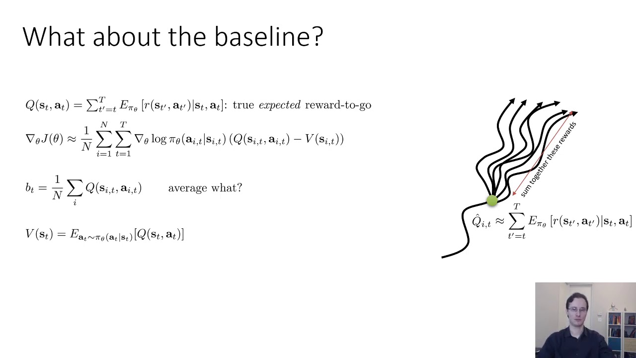
that is it's the rewards from now until the end of time which means that it refers to the rewards that you have yet to collect basically all the rewards except for the ones in the past or the reward to go and we sometimes use the symbol q hat i comma t to denote the reward to go now take a moment to think back to the previous lecture where we also use the symbol q the reward to go q hat here actually refers to an estimate of the same quantity as the q function that we saw

in the previous lecture we will get much more into this in the next lecture when we talk about extra critical algorithms but for now we'll just use a similar symbol with a hat on top to note that it's a single sample estimate all right now the causality trick that i described before you can always use it you'll use it in homework two it reduces your variance there's another slightly more involved trick that we can use that also turns out to be very important to make policy gradients practical and it's something called a baseline so let's

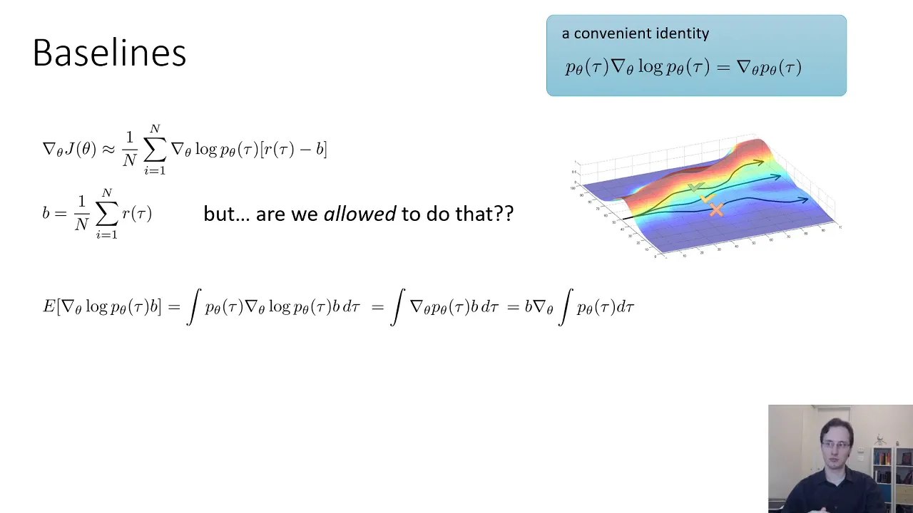
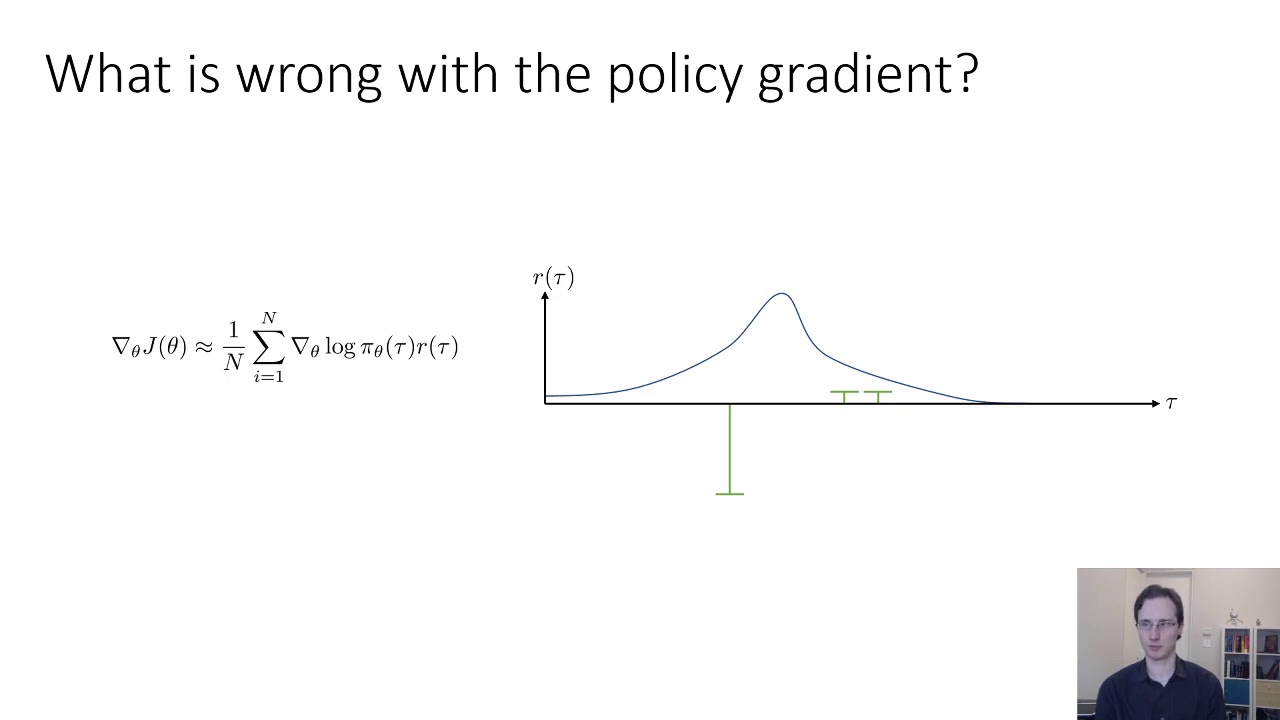
think back to this cartoon that we had where we collect some trajectories and we evaluate the rewards and then we try to make the good ones more likely and the bad ones less likely that seemed like a very straightforward elegant way to formalize trial and error learning as a grain ascend procedure but is this actually what policy gradients do well intuitively uh policy gradients will do this if the rewards are centered meaning that the good trajectories have positive rewards and the bad trajectories have negative rewards but this might not necessarily be true what if all

of your rewards are positive then the green check mark will be increased its probability will be increased the yellow check mark will be increased a little bit and the red x will be also increased but a tiny bit so intuitively it kind of seems like what we want to do is we want to center our rewards so the things that are better than average get increased and the things that are worse than average get decreased for example maybe we want to subtract a quantity from our reward which is the average reward so instead of multiplying

grad log p by r of tau we multiply by r of tau minus b where b is the average reward this would cause policy gradients to align with our intuition this would make policy gradients increase the probability of trajectories that are better than average and decrease the probabilities of trajectories that are worse than average and then this would be true regardless of what the reward function actually is even if the rewards are always positive that seems very intuitive but are we allowed to do that it seems like we just arbitrarily subtract our constant from all

of our rewards is this even correct still well it turns out that you can show that subtracting a constant b from your rewards in policy gradient will not actually change the gradient in expectation although it will change its variance meaning that for any b doing this trick will keep your grading estimator unbiased here's how we can derive this so we're going to use the same convenient identity from before which is that p of tau times grad log p of tau is equal to grad p of tau and now we're going to substitute this identity in

the opposite direction so what we're going to do is we're going to analyze grad log p of tau times b so if i take the difference r of tau minus b and i distribute grad log p into it then i get a grad log p times r term which is my original policy gradient minus a grad log p times b term which is the new term uh that i'm adding so let's analyze just that terms the expected value of grad log p times b which means that it's the integral of p of tau times grad

log p of tau times v and now i'm going to substitute my identity back in so using the convenient ending in the blue box over there i i know this is equal to the integral of grad p of tau times b now by linearity of the gradient operator i can take both the gradient operator and b outside the integral so this is equal to b times the gradient of the integral over tau of p of tau but p of tau is a probability distribution and we know that probability distributions integrate to one which means that

this is equal to b times the gradient with respect to theta of one but the grading with respect to theta of one is zero because one doesn't depend on theta therefore we know that this expected value comes out equal to zero in expectation but for a finite number of samples it's not equal to zero so what this means is that subtracting b will remain will keep our policy gradient unbiased but it will actually alter its variance so subtracting a by a baseline is unbiased in expectation the average reward which is what i'm using here turns

out to not actually be the best baseline but it's actually pretty good and in many cases when we just need a quick and dirty baseline we'll use average reward however we can actually derive the optimal baseline the optimal baseline is not used very much in practical policy grading algorithms but it's perhaps instructive to derive it just to understand some of the mathematical tools that go to studying variants so that's what we're going to do in the next portion the next portion will go through a mathematical calculation where we'll actually derive the expression for the optimal

baseline to optimally minimize variance so to start with we're going to write down variance so if you have the variance of some random variable x it's equal to the expected value of x squared minus the expected value of x squared so we can use the same equation to write down the variance of our policy gradient so here's our policy gradient the variance of the policy gradient is equal to the expected value of the quantity inside the bracket squared minus the whole expected value squared now the second term here is just the uh the policy gradient

itself right because we know that r of tau minus b in expectation ends up not making a difference so basically the actual expected value of grad log p times r minus b is the same as the expected value of grad log p times r so we can just forget about the second term changing r is not going to change its value in expectation so it's really only the first term that we care about all right i'm going to change my notation a little bit just to declutter it so i'll just use g of tau in

place of uh grad log p of tau so if you see g at the bottom that's just grad log p i just wanted to write a short a shorter value so i know that the second term in the variance doesn't depend on b but the first term does so then in order to find the optimal b i'm going to write down the derivative d var db and solve for the best b so the derivative of the second part is 0 because it doesn't depend on b so that just leaves the first part ddb of the

expected value of g squared times r minus b squared now i can expand out the quadratic form and i get ddb of the expected value of g squared r squared minus 2 times the expected value of g squared rb plus b squared times the expected value of g squared so all i've done here is i've just expanded out the quadratic form r minus b squared distributed the g squared into it and then pulled constants out of expectations now looking at this equation we can see the first term doesn't depend on b but the second two

terms do so we can eliminate this part and the second two terms if we take the derivative with respect to b the minus two term is linear in b and the plus term is quadratic in it so we get the derivative is equal to negative 2 times the expected value of g squared r plus 2b times the expected value of g squared now we can push the constant term on the right hand side and solve for b and we get this equation b is equal to the expected value of g squared r divided by the

expected value of g squared right so i've just solved for b when the derivative is equal to zero so this is the optimal value of b now looking at this thing you could try to imagine what is the optimal baseline really intuitively well perhaps one thing that might jump out at you is that the baseline now actually depends on the gradient which means that if the gradient is a vector with multiple dimensions if you have multiple parameters you like to have a different baseline for every entry in the gradient so if you have a hundred

different policy parameters you'll have one value of the baseline for parameter one a different value of the baseline for parameter two and intuitively looking at this equation the baseline for each parameter value is basically the expected value of the reward weighted by the magnitude of the gradient for that parameter value so it's a kind of re-weighted version of the expected reward it's not the average reward anymore it's a re-weighted version of it it's re-weighted by gradient magnitudes so this is the baseline that minimizes the variance now again in practice we often don't use the optimal

variance we just uh sorry we often don't use the optimal baseline we typically just use the expected reward but if you want the optimal baseline this is how you would get it all right so to review what we've covered so far we talked about the high variance of policy gradients algorithms we talked about how we can lower that variance by exploiting the fact that present actions don't affect past rewards and we talked about how we can use baselines which are also unbiased and we can analyze variance to solve for the optimal baseline