CS 285: Lecture 5, Part 2

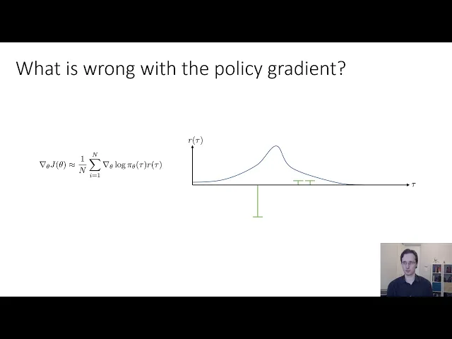
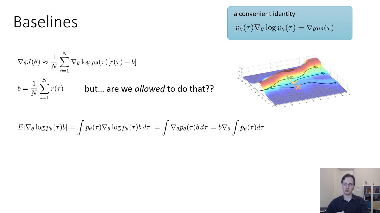
all right now that we've covered the mathematical derivation for policy gradients uh let's work a little bit on developing some intuition for what policy gradients are actually doing all right so these are the equations that we saw before we've got the approximate expression for the derivative of j theta which is a sum over all of our samples of the sum of gradlog pies along that sample trajectory times the total reward that trajectory so what is this gradlog pi thing actually well let's say that our policy for now is just a discrete let's say that it's

just a mapping from images maybe these are driving images to a discrete action turn left or turn right then log pi is simply the log probability that this policy assigns to one of those two actions and grad log pi is the derivative of that log probability so uh a neural network will output those probabilities and you can take the logarithm of that probability when you do maximum likelihood training supervised learning you're typically maximizing log probabilities of observed labels so it's instructive perhaps to compare what policy gradients are doing to what maximum likelihood is doing so

in maximum likelihood like in imitation learning for instance we would collect some data of humans selecting actions and then we would run supervised learning on that data and that would yield a policy pi theta a t given st the maximum likelihood objective or the supervised learning objective is just a maximization of the log probabilities assigned to the observed actions so the gradient of that is given by the sum over all of your samples and all your time steps of grad log pi a i t given s i t now of course when we're doing maximum

likelihood we assume that the actions in our data ait are good actions to take in policy grading that is not necessarily true because we generated those actions by running our own previous policy which might not have been very good so the maximum likelihood gradient simply increases the log probabilities of all the actions whereas the policy gradient might increase or decrease them depending on the value of their reward so intuitively high reward trajectories get their log probabilities increased lower board trajectories get their log probabilities decreased so you can think of it as a kind of weighted

version of the gradient for the maximum likelihood objective in fact this interpretation will turn out to be very useful when it comes time to actually implement the policy gradient with modern automatic differentiation tools like pytorch now that was an example with discrete actions what if we have continuous actions what if for example we want to make this little humanoid robot run using policy gradients well in that case we need to select a representation for pi that can output distributions over continuous valued actions for example we might represent pi theta a t given st as a

multivariate normal distribution or gaussian distribution where the mean is given by a neural network so the neural network outputs the mean and then you have some variance which could be learned or could be fixed and then you would like to train this neural network in that case you can write the log probability as uh you know by basically using the formula for the log probability under a multivariate normal distribution which is simply the difference between the mean and the action under the covariance the inverse covariance matrix so this is one way of writing the log

probability of a multivariate normal distribution and you can then calculate the derivative of this thing with respect to the the mean and you just get this equation so the derivative of your multivariate normal is just negative one half times the inverse covariance times fst minus a t times df d theta and in practice the way that you would calculate this quantity is you would compute negative one half sigma inverse of s t minus a t and then back propagate it through your network to get the derivative with respect to theta all right so that maybe

gives us some intuition for what these grad log pi terms are actually doing both in the discrete action and continuous action case in both cases they correspond to a kind of weighted version of the maximum likelihood gradient if it's helpful for you to think about it that way and you can compute them by basically using the formula for the log probability of whatever distribution class you choose to use now what is the policy gradient actually doing intuitively um so i'll collect some of the terms and and use slightly more concise notation to make this little

clearer so you can equivalently write it as grad log pi theta of tau times r of tau uh where this grad log pi theta tau is just the sum over the individual grad log pi thetas the maximum likelihood gradient is given here so it's just the same thing only without the r term so intuitively what that means is that if you roll out some trajectories and you compute their rewards and some of them have big positive rewards represented with green check marks and some have big negative rewards represented by the red x and some are

kind of neutral like that middle one what you'd like to do is you'd like to take the log probabilities along the good trajectories and raise them and take the log probabilities along the bad trajectories and lower them so the policy gradient makes the good stuff more likely and makes the bad stuff less likely so in a sense you can think of the policy gradient as a kind of formalization of trial and error learning if reinforcement learning refers to learning about trial and error then policy gradient simply formalizes that notion as a gradient ascent algorithm now

what i would like to briefly mention next is a short aside regarding partial observability so if we want to learn policies that are conditional observations rather than states the main difference is that states satisfy the markov property whereas observations in general do not as a reminder the markov property simply says that future states are conditionally independent of past states given present states states satisfy this whereas observations in general don't now interestingly enough when we derive the policy gradient at no point did we actually use the markov property which means that if you want to derive

the policy gradient for a partially observed system you could do so and you would get exactly the same equation now for a partially observed system the trajectory distribution now would be a distribution over states actions and observations and you have to marginalize out the states so the derivation for this is a little bit more involved but you can do it at home however if you follow through that derivation you will end up with exactly the same equation that we got before only the s's will be replaced by os what this means is that you can

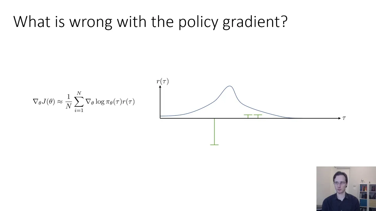
use policy gradients in partially observed mdps without any modification just just use them and for this version of the policy gradient algorithm it'll work just fine insofar as regular policy gradients work okay now i mentioned before that maybe policy gradients as i've described them so far won't necessarily work very well if you actually try to implement them so what's wrong with a policy gradient well uh here's one one uh problem that we could think about uh let's say that the horizontal axis here denotes the trajectory and i know the trajectory in general is not one-dimensional

but let's pretend it is and the vertical axis represents the reward so here we have a reward it's kind of this belt curve shape with a peak here and let's say that we have three samples and the height of the bars here represents the the reward of those samples so the blue curve shows the probability uh under the policy that's the bell curve and the green bars show the rewards so i apologize here the y-axis is actually a little bit overloaded it's showing both rewards and probabilities so the blue thing is a probability it's always

positive the green stuff is the reward which may be positive or negative okay so with these three samples we could now imagine when we calculate the policy gradient which way will the blue policy distribution move which way will the trajectory distribution move so take a moment to think about this now the policy gradient you can think of it as basically a weighted maximum likelihood gradient so we're going to take each of these three points and we're going to calculate log pi at each of these three points and we'll multiply it by the value of the

reward so the sample on the left has a very negative reward so we'll try to decrease the log probability there and the two samples on the right have small but positive rewards so it will somewhat increase their probabilities so that means that the policy distribution will slide to the right and it will mainly try to just really avoid that big negative sample now we know that if we take the reward function in mdp and we offset it by a constant meaning that we add the same constant to the rewards everywhere the resulting optimal policy doesn't

change right uh this is for the same reason that if you have a maximization problem uh let's say you're maximizing f of x the maximum for f of x is the same even if you add a constant so the maximum for f of x is the same as the maximum for f of x plus 100 which is the same for f of x plus 1 000. so let's add a constant to the rewards so let's say that our rewards are now given by these bars now the relative rewards are exactly the same so the samples

on the right are still better than the samples on the left but now i've added a cost to them so they're all positive and now take a minute to imagine how the policy will change when we use these rewards with these rewards of course the policy will want to increase the log probabilities at all three samples although it will want to increase the ones on the right a bit more so maybe the policy will change like this now you could imagine even more pathological changes to the reward uh what if i for example change the

reward so that the two samples on the right actually go all the way to zero or the sample on the left goes to zero this issue is actually an instance of high variance essentially the policy gradient estimator that we've described before has very high variance uh in terms of the samples that you get so depending on which samples you end up with randomly you might end up with very different values of the policy gradient for any finite sample size now as the number of samples goes to infinity the policy gradient estimator will always yield the

correct answer so this issue with adding constants to rewards will not make any difference but for finite sample sizes they will and this makes policy gradients very hard to use it means that in practice in order to make policy gradients be an effective tool for reinforcement learning we must somehow lower this very high variance and a lot of advances in policy grading algorithms basically revolve around different ways to reduce their variance and we'll cover some of those in today's lecture so you can think of an even more pathological version of this issue if some of

the samples have a reward of zero then their gradient basically doesn't matter at all and in general this issue doesn't go away completely as you increase the number of samples but it ends up being greatly mitigated all right so to review what we've covered so far we talked about evaluating the rl objective with samples we talked about evaluating the policy gradient where we have to use this log gradient trick to remove the terms that we don't know namely the initial state probability and the transition probability and then we can again evaluate the policy gradient using

samples and we talk about how we can understand the policy grading a little bit better intuitively by uh treating it as the formulai the formalization of trial and error learning into a gradient ascent algorithm we briefly talked about how policy gradients can also handle partial observability and then lastly we talked about why policy gradients might be hard to use so in the next portion of the lecture we'll try to address this