Lecture 22: Stein

So i chose this topic because um i think a lot of people don't see it even a lot of the stats phds don't see it i think it's one of the coolest and most beautiful results in statistics so i personally like this very much and i think it's very good to see at least once um and it's very is a very influential result that there's a lot of Applications for it so we're going to spend the week on it a lot of the popular suggestions were active learning that was one of them and then actually

i'm not sure why we decided to do this but larry's going to give a tirade so next week is going to be monday is going to be active learning because that was one of the most popular topics so we'll give you an active Learning brief and then wednesday larry's just going to go on a tirade that's what we're going to call it and was that a suggestion that he made i'm not sure if he so he's going to tell you about how he doesn't like all the assumptions that people use in theory so he's going

to go through all the assumptions he finds offensive and just tell you why he finds them offensive and how you can get around Them so we've been using a lot of assumptions so far this semester right maybe that's why we chose it um so that'll be the end of class then so active learning then tyrade um so stein's stuff uh stein is a very interesting guy how many of you guys have heard of charles stein before just curious so what would you have heard of him for About stein's llama okay well they're they're actually like

three or four stein's limits so i'm not sure if it's the exact same one but but stein was um they're all related so it's very likely that this some of this sounds familiar stein is still alive he's at stanford uh he's about 90 i'm guessing 94. he's pretty old stein in many ways shaped the landscape of statistics post-world war ii So uh this result we're going to talk about came from a 1981 paper that he wrote um stein wrote very few papers i think he's written something like 20 actual journal papers over the course of

his career which is remarkably little considering somebody who's 94 and has had such a big influence on statistics and there's this kind of uh you know there's this thought some people say which is let's you know with All the papers being written today could you imagine would be like if somebody told you you could only publish 20 papers in your life it was like your life's limit and you're only allowed 20 so once you get to that point you can't publish anymore that would be a very different way of doing things right research-wise but you

know stein probably wrote uh per paper he's probably the most influential Person i can think of in statistics so he he really met that quota and he did a lot and the interesting thing about this paper is that it was actually written a lot earlier in 1981 so it's evidence that stein knew about this result even in the 50s and 60s so he wrote papers that kind of referred to this result earlier but he never published a paper on it until 1981 and actually in 1974 Um the rumor is that he actually wrote this paper

and he thought it wasn't good enough when he actually put it in his desk just put it away in his desk drawer and one of his colleagues at stanford who closed his collaborator um happened upon this paper maybe he was on his uh you know on this front desk or somebody said can i read this and you Read it and he was just amazed he said you have to publish this and stein said no he doesn't think it's important enough maybe he thought people already knew it and so what the paper that appears in the

statistics 1981 it was actually in in large part written by someone else it was stein's paper that was that one of his colleagues took and decided to this is the rumor decided to kind of Reshape it into a journal paper and put it out in his name so it's it's pretty amazing when you think about all this the uh you know the impact this papers had given kind of all the the caveats i just said to you and it starts off with a very simple observation and we're going to talk about this the implications of

this observation for Unbiased risk estimation that's going to be the focus of this this week's lectures stein's lemma the one we learn actually has a converse so that might have been one you've heard in probability theory if you've taken advanced probability theory the converse has a huge number of implications in probability theory so this lemma is is very central to kind of a lot of important work in statistics and Probability let's just get to the um the basic univariate result it's very simple to state which is that this is what i would call stein's luma

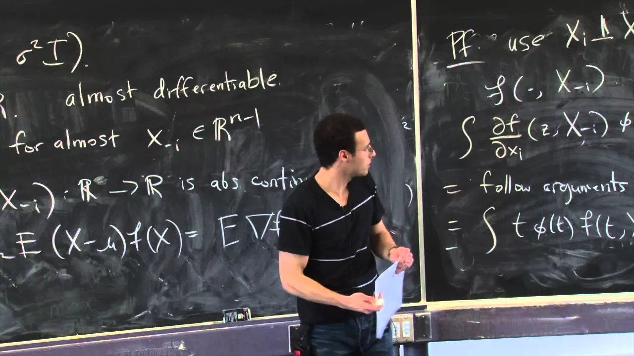
and is that if we have just a univariate normal random observation okay z comes from standard normal and you give me a function that goes from r to r And we're going to assume that it's absolutely continuous so for those of you who don't know what this means that's fine just think about it like differentiable continue us okay so think about it like f is differentiable and or maybe it's differentiable almost everywhere something like that it only has a finite Number of discontinuity points okay if that's true then this is stein's lemma it's very simple

fact the expected value of z times f of z is equal to the expected value of f prime of z Okay so because it's absolutely continuous its derivative exists almost everywhere so this is kind of uniquely defined that's stein's lama so this is what you saw in another class before this one okay so the the converse to this is actually true in the sense that if let's suppose this holds For all absolute continuous functions that implies that z is normal zero one so this property is a characterizing property of the normal distribution if this is

true for every every absolutely continuous function it must mean that z is normal and that property has uh like i said that has a lot of implications in probability theory so stein's lemma is used in probability theory to prove convergence to normality There's a a a whole almost course you could teach in fact i think we don't quite do it yet but we had a a whole semester-long reading group we spent maybe his last year on stein's lemma and probability theory we're going to learn the implications of this direction this week so we're going to

first prove this so you you can see how simple this really is Intuition uh honestly i i this is not a situation which i can give you a lot of intuition it comes right out of the property of the normal density the derivative of the normal density is equal to minus c times the normal density right if you differentiate phi of z because e to the minus c squared over Two right so i i don't know if i can give you much intuition beyond that the fact this is true for normal distribution and only normal

distribution if it's true for every function that was a very kind of surprising result i don't think there's a lot of intuition behind that either but it turns out there's actually a Characterizing equation there's a stein equation for other distributions as well so for poisson random variables there's a stein equation what people discovered for other random variables there's a stein equation so this happens to be the one for normal the normal distribution so let's let's prove this um well we're going to do it in two ways actually the first way is going to be integration

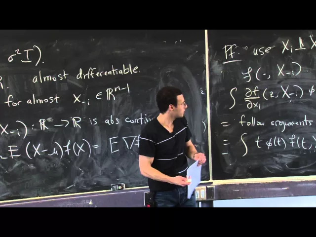
by parts So this is proof one and the second way is going to be uh a little longer proof but the longer proof we're going to see is useful when we talk about the multivariate version of this because the multivariate version of this i guess is easier proved from the longer version of the proof so let's just go with the the left-hand side right the left-hand side is equal to the integral Oh sorry we're gonna start with the right-hand side it's the integral of f prime of z phi of z dz right where uh this

is the normal density and that's it's our function f that's the derivative of our function f prime and let's use integration by parts right integration by part says that this is equal to The product of these two evaluated between minus infinity and infinity and i have to subtract off f of z p prime of z dz okay so first of all this is zero because this goes to zero at either ends right infinity to minus infinity so that this whole term is zero Because because of the normal density now what's this term well that term

well it's the property i just said before right so phi is equal to you know e to the minus c squared over 2 divided by root 2 pi and z squared over 2. and if we differentiate this we get that V prime of z it's just equal to minus z times this right so it's equal to minus c times phi of z so let's use that and we just see that we get uh you know z times f of z times v of z dz pretty pretty simple right very simple proof and that's exactly the

right hand side the expected value of The left-hand side sorry we started the right-hand side we worked our way to the left-hand side the expected value of z times f of z okay hopefully that's clear let's do proof two so proof two i guess i'm gonna start down here just a little bit longer and we'll go to that board it's really the same argument almost it's just that it's written differently So it's not it's nothing really uh too challenging about it so we again to start with the right hand side and now we use the

fact that this is equal to the integral of the derivative of the normal density from minus infinity to z right fundamental theorem of calculus i can Always write a function as the integral of its derivative from say minus infinity to the point which i'm evaluating it so i can always write this as f prime of z times the integral from minus infinity so if i'm leaving off the bounds it means just from minus infinity to infinity minus infinity to z Of say fee prime of t dt dz right what this is um this i can

write as uh minus t times phi of t just from the property of we just said right here p prime of t is minus t times phi of t and now i'm going to split this up so I'm going to split this up over the parts where z is positive where z is negative so this is equal to the integral from 0 to infinity of f prime of z times the integral from so this is actually going to be minus infinity to z With a minus sign but i can actually i can get rid of

this minus sign and just flip the signs flip the bounds here right and so i get z to infinity of t times phi of t dt and then the second one i'm going to leave alone minus infinity to 0 p prime of z times integral from Minus infinity to z of t times v prime of t dt dz okay um so hopefully we're all clear here i just all i did is i split this integral up over this domain where z was positive neg positive and then negative and now i'm going to apply uh fubini's

Theorem right so if i'm integrating over all the set of all z for which z t pairs for which z is bigger than equal to zero and t is bigger than equal to z i can rewrite that right as a set of all uh t being bigger than equal to zero and z being less than or equal to t and the same thing down here so i'm just this is uh just applying a Re-parametrization basically fubini's theorem so i'm going to first integrate over t so all positive t t bigger than equal to z of

this quantity and then i'm going to integrate over all z that are smaller than equal to t of this quantity dz dt and the second thing for the other integral Okay can you guys all see that so i just use fabini's theorem there and now again i apply the fundamental theorem of calculus that's really all that comes down to it right which is that if i integrate the derivative of a function over two endpoints i get the function evaluated at those two endpoints that's all it is so i'll erase proof one and just continue Up

here so let's just evaluate that that's integral from 0 to infinity t phi of t of we get f of t minus f of 0 dt minus minus infinity to 0. t P of t f of 0 minus f of t no sorry f of z that was right f of t dt and these terms cancel right so this term well actually if i combine this term see this term say with this term You'll see that they cancel because by symmetry of the normal distribution these are the same thing and if i combine the other

terms i should get right i get from 0 to infinity t phi of t f of t then i get plus because there's two minus signs from infinity to zero t phi of t f of t and so all that's left over is the integral of t phi of t F of t dt that's proof two so this is the one in stein's paper but it's not i think you know the easier proof i think was just skip because the multiversion is harder to prove that way yeah oh that's right but see i then then

i re-parametrize this is this function um Right i take i just called minus t u or something like that so i used kind of a re-parametrization here as well are you talking about this step from here to here from to this thing yeah so i thought the limits i get z going from uh integral going from z to minus infinity i i should have now t Phi of t dt then call u minus t and so that then it should work out right so then i'm going from yeah actually that's another way to see it

right any other questions okay so this point this looks like maybe a you know a little nice toy lemma something that you tell your friends to impress them about Why statistics is cool but or maybe not but um nothing maybe super substantial right we're talking about a universe normal distribution so it's a property of of normal zero one but um we're gonna go let's talk about a corollary now um i guess i'll go over there corollary of this result We get immediately it's quite nice which is that let's suppose x is normal with mean mu

and variance sigma squared and f is again absolutely continuous by the way the precise definition of absolute continuity is exactly this one so it's just that a function is absolutely continuous if i can ever take the integral of its derivative and it Gives me back the function at the endpoints so a function is absolutely contains if there exists a function which we'll call f prime for which i can apply the fundamental theorem of calculus so that's how we used absolute continuity so differentiable functions are absolutely continuous and this is a little bit more broad because

you you can suppose suppose f prime didn't exist at some point That would still be okay we can still form this integral if that had just you know le bag measure zero or something so that's why we're saying absolute continuity um so let's suppose x is normal with mean mu and variance sigma squared then actually i claim that this result is true if i take 1 over sigma squared times the expected value Of x minus mu times f of x then that's equal to the expected value f prime of x okay so this is this

is the corollary of that where does that come from let's just define z to be equal to x minus mu over sigma and let's just define the function it's called f tilde at a point Z to be f of sigma z plus mu and now let's apply this result to z and f tilde tells us the expected value of z times f of z is equal to the expected value of f times sorry f tilde of z is equal to the expected value of f tilde prime of z okay um well z remember was X

minus mu over sigma so that's where we got this if we only had one of them times f tilde of z but f told of z is just f of sigma z plus mu which is x and uh that's equal to the expected value of f tilde prime of z according that result which is equal to well we use the chain rule we see that That we get a sigma times you know the derivative of this function evaluate at sigma z plus mu but that's x again and we move the sigma to this side and

that gives us this result so that's all we've done let this be true and apply the previous result so all of a sudden we've gone from being I think a parlor trick to something that's actually really pretty interesting um which is that let's take a look at this what is this expression right here this is equal to uh let's say the the covariance is the covariance of x and f of x so we said the covariance of x And f of x once we divide by sigma squared is equal to the expected value of f

prime of x let's suppose we knew that z was normal x is normal we didn't know its mean and f of x was some function that was complicated some complicated function and i want an estimate suppose i want to estimate this Don't know the mean of x but i want to estimate the covariance of x and some complicated function of x f x well how would i get an unbiased estimate of this the covariance is equal to right equal to either the expected value of x minus mu times f of x that's one way to

write it another way to write it is this equal to the expected value of x times f of x minus its mean Expected value f of x right both those are two different ways of expressing the covariance or of course it's the expected value of x minus mu times this well how do i estimate this if i don't know the mean because if i want an unbiased estimate of the covariance of force that would suffice if i knew the mean i observe x i subtract off mu and i Multiply that f x that's an unbiased

estimate of the covariance but if i don't have a mean that's not a feasible estimator and how about this well um to get an unbiased estimate from this representation of the covariance right i have to take my observed x multiply by f of x minus its mean but if f is complicated this is very hard to compute furthermore this is Going to depend on mu right the expected value of f x is going to depend on mu so i cannot get an unbiased estimate of the covariance unbiased one directly if i don't know the mean

but what stein is telling us that let's suppose that x was normal even if you don't know a mean it's mean it's normal then this gives you an unbiased estimate Of the covariance i just differentiate my function and evaluate it at x that's and unbiased at some of the covariance i mean once i multiply it by sigma squared so the amazing thing is it doesn't depend on you okay you can guess where we're going to want to estimate covariances when we start talking about risk estimation if You remember our decomposition for risk in terms of

training error the covariance popped up very naturally just came came right out and that's where we're going to use it to do unbiased risk estimation i think that's that's a kind of very important aspect of this so before we get to risk estimation we have to talk about the multi-right version of the lemma And i'm not sure whether it's worth proving it the proof really is very similar to proof technique number two i don't know we'll see i'll just state it first at least so the multivariate version says the following let's suppose that x is

a multivariate normal with mean mu And covariance matrix sigma squared i now the fact that this is spherical is actually really important um you'll see well at least i'll go part through part of the proof and you'll see why it's important so this is very important that the components of x have a spherical covariance and let's suppose that F is a function that goes from now rn to r so x is in rn so mu is an n-dimensional vector and i is the end by an identity matrix and s this function stein calls almost differentiable

and so if those of you uh who've taken functional analysis before maybe look at this definition you Might think it looks like the definition of weak differentiability so they're very closely related but this is just something stein made up all it means is that for each eye and for almost every x i'm going to write it like this minus i that's an rn minus 1. so this is a point where if i'm fixing N minus 1 of its components so almost every means with respect to le veg measure for almost every point x minus i

this function f with all the other components fixed at minus i so x minus i what i mean by this is that this function f is a function of n variables i'm thinking about as the as a function only of the ith variable with All the other components fixed at x minus i so this is a univariate function right from r to r this function has to be absolutely continuous sorry this goes from r to r this must be absolutely continuous so think about this meaning it's basically differentiable okay so it maybe seems like a

weird definition but think about it in the Following way if i take any uh line that's parallel to the coordinate axis so i pick one chord axis pick uh coordinate axis i take a line that's parallel to it it's defined by this and along that line f has to be absolutely continuous so the function has to basically just be differentiable along that line pick any line pale of the coordinate Axis in any coordinate axis and actually it's not even any line it's almost every line right if i take some slices and it happens not to

be differentiable that slice that's okay just can't be um you know as many slices to constitute something of non-zero measure so really it's just almost every line so it's well behaved along the Directions parallel to the coordinate axis then stein's lemma so let's assume all this x in this function stein's multivariate lemma says that one over sigma squared times the expected value of x minus mu times f of x so let's just inspect this look this is Actually in r this is an rn so i'm just taking this and i'm multiplying by every component of

x minus mu this is equal to well you can guess what it's equal to right based on the universe version it's just the gradient of f at x that's stein's multivariate lemma from for a multivariate Normal random vector okay again it's it's quite amazing because um this is something that's computable you give me a single observation if i know my if right now my function i compute it's gradient this is computable this is an unbiased estimate for this quantity which if you try to estimate in any other way pretty much it's going to depend on

mu which you don't know this of course doesn't depend on you you Give me an x i compute the gradient of my function and that's it uh let me just at least mention the the proof the ideas of the proof maybe we won't go through all of it so we have more time for uh applications but the proof is is not much harder than the one we just did the unibright version so the the proof uses the fact that um so we're going to use the fact that x i And x minus i are independent

and that's true because of this spherical normal distribution right so they're we know that since the they have no covariance and they're normal that means that they're actually also independent so this is important for the proof i fix all the other components of my normal random vector this one is not affected in terms of this distribution And therefore we're going to look at this function f of x minus i and in fact i can uh i can think about even just conditioning on this this condition on the value of x minus i and apply basically

the arguments of stein's univariate um Lemma and if we do that we're going to see that the right the partial derivative of f with respect to variable i the i component of its gradient say if i evaluate this at z comma x minus i phi of z dz then that's going to be the ith Component of this right i'm taking the i component of the gradient or it's it's partial derivative conditioning on the value say of x minus i i'm integrating with respect to x i just follow the arguments that we did before there's no

difference just ignore that and close your eyes if you don't want to see that big x minus i And you'll see that it ends up being equal to same thing we had before t phi of t f of t comma x minus i dt and the reason that we went through that kind of more complicated argument using fabini is that it happens just to be easy to apply absolute continuity in that argument remember because absolutely continuous meant that if i Integrated the partial derivative or the derivative of the function from one endpoint to another it

was equal to the difference between the function valid at those two endpoints and here um the assumption is that that's true if i fix all the other arguments and look at f as just a function of its ninth argument that was our assumption that it's almost differentiable along that line so that's just exactly where it comes into play in the proof And uh right what we've shown in other words well we can actually see it from here we've just shown that uh if i take this and condition on x x minus i then it's equal

to this the i component of this condition on x minus i right think about all i've done here is i've conditioned on the value of x minus i you can make It a lowercase x minus if you wanted to think about as conditioning and i've shown that this side and the i component condition on x minus i is equal to this side and the i component on x minus i and then if it's true conditionally it's true unconditionally too just integrate over x minus i and i i've established the either quality here and there's nothing

special there about The either quality questions about that part yeah i'm not sure um well i mean that's it's not a bad question um certainly not so first of all if we had an unbiased estimator from u then it wouldn't be the case that we'd have an unbiased estimator for mu Times f of x my expectation is not uh linear so i wouldn't necessarily have a number assessment for this anyways second of all suppose i'm in a setting where it's actually quite hard to do that or i don't have good estimates of mute that's really

we're going to use this for so the goal the goal the other day is to estimate the mean that's going to be the older of our estimation problem and in Some part of us stand mainly mean we need to estimate this thing now if we assume that we had an estimated mean estimate this thing it's kind of circular we're trying to assess maybe the quality of our estimate of the mean even that we that we have that's a good question though other questions so let's make a final remark And then we'll take a short break

and we'll see what we've done or maybe i'll just i'll do it all at once and then you can take a short break afterwards so what's the final remark maybe i should have written that in different notation so it's not to confuse you but let's suppose now that i have x that's normal with mean mu And covariance sigma squared i and i have a function f that goes from rn to rn so we're stepping up once more we're going kind of more and more complex in terms of what we're studying and f i can write

as f1 through fn where each of these goes from rn to r so these are its coordinate functions right each of these goes from rn to r And let's suppose that f is almost differentiable which means all it means is that each one of these guys is almost differentiable okay f1 through fn are all almost differentiable so it's a nice function if i look at any chord line compelling to the coordinate axis and look at anyone's component functions then they all basically have derivatives There then we can actually apply stein's lemma to this function just

by applying it component wise for each one of these so all i'm going to do is look this is actually a set of n equalities right because this is n-dimensional it's n-dimensional i'm going to apply this to each one of these functions f1 through fn and When i look at the equality for say fi i'm just going to take the i equality here so i'm going to from stein's limb i'm just going to conclude that there's no need to prove this because it's kind of immediate what i'm saying first of all steins lema tells us

this is true if i look at f i of x Is equal to that's true for all i that's just applying that each one of the component functions and now i'm just saying let's just take the ith component of this equality there's n of them so all i got to do is look at x i and mu i that's the ith component here and look at the earth component of the gradient here So stein actually tells us that's true we've actually lost some some stuff there right we've we have more equalities than this but we're

just throwing them out we're not even considering them so this is true and therefore it's true if i sum it up so in other words the sum let's sum over all i from i equals 1 to n That's equal to the sum here of the expected value well maybe i'll write the sum on actually on the inside but it doesn't matter and again i can actually the same thing here i'll write the sum on the inside but it doesn't really matter okay i've just taken the sum basically on each side of the equality And now

this should start to look very familiar what have we proved here we proved that 1 over sigma squared times what is this this is the covariance between x i and f i of x so the sum of the covariances between x i and f5 of x is equal to well there's not really a great expression for that other than what we Wrote down this is called the divergence of f we may write it a little bit differently like this but it's equal to the sum of the partial derivative of the i-component function with respect to

the i-variable evaluated at x what is that right that's the degrees of freedom so Let's think about f why do we think about f in this framework it's because we're thinking about f as taking in an observation and dimensional observation and producing an estimate of of the mean of x let's think about that f is our favorite most complicated estimator and you give it an a normal vector it does very complicated things and produces a mean An estimated meaning of the normal vector right this could be linear regression it could be something very fancy it

could be you know something non-parametric it can be whatever you want it just takes in um say we usually think this is y so takes in say y instead of x just so you can get your bearings and produces out mu hat Our estimate of the mean or y hat this is saying that the degrees of freedom of that estimator all right the covariance the sum of the covariances between the ith observation this is the ith fitted value what we would estimate is equal to something else that's something else is the expected value of the

divergence of our function and now we're going to just do a little Bit of refresher as to why this is so kind of important slash remarkable a remarkable result of stein something we did i think on my first lecture we talked about this the very first lecture i gave maybe the second lecture of the course which is if we take if we take our estimator mu hat all right let's let's call mu hat All right up here mu hat is f of x so you give you give me x i'm gonna f could represent some

very complicated even optimization problem i solved to get an estimate of the mean and i want to know the risk of my estimator so how what's the expected square distance between mu and mu hat then we did this in like i said the very First class i think even we can actually expand this out as follows oops i guess i switched to y so maybe i was also b loaded by the x here okay so maybe we more typically think about it as y observation vector so i'm just going to form this very simple risk

expansion Which we already did already i'll just skip the details expand this out details on the notes you'll see that i get n sigma squared that's for this guy plus expected value of y minus mu hat squared so the second guy and the cross term after you work it out is exactly equal to this 2 Times the sum of the covariances between y i and mu i hat what is that look that's just what we have here we call this degrees of freedom or actually this is sigma squared times the degrees of freedom of mu

hat and is this a term you don't have to remember it that way but it's helpful to remember it by name We also have some interpretations for it like it told us the effective number of parameters that mu is using when it estimates y and what did stein tell us he told us that actually this is exactly equal to provided that this function f is nice it's equal to the following two times the Sigma squared times the sum of the divergence or the expected divergence this is the expected value the sum of if we differentiate

our estimated respect to y i and add that up and we'll go through a few examples so you can get an idea this may look a bit uh obtuse or something But you'll get a sense of that this can be easy to do in many cases okay so still so far looks like we just exchanged one maybe expression for another but here's where the unbiasedness property is so important there's a very easy unbiased estimator of this whole quantity right what is it let's take r hat let's call this r that's the risk we're trying to

estimate R hat i'm just going to take to be i can forget about the sigma squares because usually i don't care about the risk up into a constant if i'm trying to say minimize the risk over some tuning parameter but let's suppose we knew sigma squared for now then i'll just form this unbiased estimate right by stein's lemma Not really by this representation for the risk it is so uh it holds that the expected value of r hat is r you can just see it directly from comparing these two equations so this this r hat

is called sure stein's unbiased unbiased risk estimate that's that particular form of risk estimate Questions about about this right so i think in the first few lectures i was saying that we have if we can evaluate the degrees of freedom then we can get an estimate like suppose i had an unbiased estimate for degrees of freedom so i had an unbiased estimate for this quantity then i said well then we could form an unbiased estimate of r in the same manner I was actually talking really about this because most of the time our estimates for

degrees of freedom come from this divergence in some cases we can evaluate them explicitly like for linear smoothers we saw we can actually evaluate this term explicitly but in general this is a much more broad way of doing it okay um So i'm not going to write it down but i'll just say it out loud uh it should be kind of intuitively obvious to you now that if mu hat depended on the tuning parameter suppose i wrote this as mu hat of lambda then if i want to choose lambda i could try to minimize this

overall lambda right if i if i wanted to choose a tuning parameter in some way then one way to do it is to write down Stein's unbiased risk estimate as a function of the tuning parameter and then choose the tuning premium to minimize that risk estimate that's something people do quite often actually in order for that to be successful there needs to be two things to happen the first is that you need to be able to compute this if you can't compute this for your estimator then you can't use sure You have to be able

to compute this diversion so i'll give you some examples of where you can do that the second thing is is the more subtle thing and this is where this connects to what things you've learned already actually even this part connects to things you've learned already but the second thing is more subtle which is that we have to know that somehow by Minimizing r hat as a function of lambda that the resulting estimate are still going to have good risk right so let me write it down over here let's suppose i were to take r hat

as a function of lambda minimize it over all lambda in some set in most applications it would be prudent to then want to say to want to prove that this has a good risk property just Because you minimize the unbiased estimate of the risk doesn't mean that its risk is actually good like we would like to say somehow right that r of lambda hat is good maybe r of lambda hat should be close to the minimum of the true risk that would be kind of the eventual goal right or even r of lambda hat should

be close to r hat of lambda hat If you want to say something even kind of closer because that's what we see we minimized our unbiased test of the risk it gave us our risk was this number and we want to say well what is the true risk how different is the truest from that number so what does this remind you of that we learned recently right so concentration and measure is exactly what you'd have to use here in order to make sure that this thing concentrates Around its expectation uniformly over lambda if we could

show that then we'd be confident that even if we evaluated r hat lambda hat that would be close to r of lambda hat which is the expectation right at any fixed at any fixed lambda r hat of lambda's expectation is r of lambda so a little bit of um history of what happened after this paper and then i'll take a break is that when this paper Came out there was an explosion of interest in this kind of thing and this relates by the way to things like aic bic they're very related to this but this

in a sense is i don't want to say more broadly applicable because um aic and bic each have their own motivation that's kind of beyond the simple forms you see them in regression but this is a very general Idea right all i need to do is be able to differentiate some function and i get a very kind of general class of unbiased risk estimates so there's a ton of interest in this and also connecting it to things like aic and bic and cross-validation and the first wave of papers all looked at simple estimators where this

was easily computable and they gave Concentration arguments like this so they said for things like spline smoothings other simple procedures we can use this to minimize the to choose the tuning parameter and we can be confident that the risk of that resulting uh you know adaptively selected model is good and i gave i think five references here um six references so there's a but these are just six of Many there's kind of explosion of of interest in this nowadays uh people still are interested in stein's unbiased quest estimate but they've kind of forgotten this part

they don't do this concentration argument anymore and i have to say i'm also guilty of this i i've worked on some stuff related to this and i i you know the papers that i've worked on do not consider concentration And the the reason is because uh when you think about really complicated estimators actually all the work goes into computing this so beyond simple estimators like linear smoothers or other simple ones you've learned you know you can write a whole paper on just computing this divergence concentration then becomes very complicated because you're asking for a Very

complicated function r hat to concentrate around its mean so i listed i think another eight ten papers written recently that all focus on computing this for different things so there's uh some for for the large algorithm some for the lasso some for convex constrained regression estimators reduce strength regression Singular value thresholding hierarchical base modeling so all these papers focus on competence divergence for different estimators and then they they kind of skip this part because it's maybe too hard um so yeah so my plan was for the rest of the time was to give you examples

of this where you can compute this and what it means And then to give an example of where we can prove that it concentrates just to show you kind of both sides of the of the story let's take a quick break though and we'll come back and do the last 20 minutes or so um all right let's this is a definitely a fun topic so let's cover this one and And if it spills over next time we can see how much we want to talk about it so science paradoxes um in many ways i think

it's kind of like the birth of regularization uh you know i'm continuing to say the same thing over and over again but stein was a very influential guy and he he had this idea which is a very big one and he also had the idea that Shrinkage was a form of controlling the variants which enabled better estimation which kind of i think in many ways is you can think of it as as leading to modern regularized estimation all the fancy forms of regularization that we learn now and he has this very surprising result people call

stein's Paradox or at least i call it science paradox i don't know unfortunately stein has a bunch of lemmas and so they're all referred to as stein's lemma so i'm going to call this one stein's lemon i'll call this result stein's paradox and it starts off in the setting so x is normal mu sigma squared and it's an rd i mean rn rd doesn't matter But let's just call it rd for now and uh in other words just to be perfectly explicit i have d normal observations they're independent they each have different means okay so

d observations independent each have different means let's before we talk about the paradox let's establish the ideas of Admissibility and intimacibility this is maybe something you learned in 705. i'll just remind you of what it means so um we say that uh let's call it let's say immense ability first so theta say some estimate of theta hat suppose it we're estimating some quantity theta Somehow i really messed up the notation here in the my notes sorry about that i'm mixing up theta hat and mu so let's just stick with one of them let's say mu

hat so mu hat is our estimate say for mu it doesn't need to be in the normal problem in any problem i just have an estimate you had of some other quantity mu and we say that new hat is inadmissible so it's in Admissible if there is some other estimates called mutilda such that the following holds we have another estimate that has risk that's no worse than that of mu hat this has to be true for all mu so no matter what the true parameter was That we're trying to estimate uh we do no worse

if we take mu tilde versus muhat and one other thing has to hold we have to have strictly better risk so has to be strictly less than that we get from you had for some u it could even just be one mu right so it's never worse and at some points it's strictly better If this happens if if you give me a mew hat and i can find a mutilda with this property then we say that mutilated dominates muhat it dominates it so that means in some sense there's no reason you'd ever use mu hat

because i can always do better or i can always do no worse and i can sometimes do better depending on what the truth happens to be In this case we call muhat admissible inadmissible excuse me inadmissible and it's uh admissible if this doesn't happen so admissible means that we cannot dominate it by anything else okay so admissibility and and uh is a different concept than in than other ones that you've learned like for example um We learned when we talked about minimax theory that you know certain estimators are minimax that doesn't mean that they're inadmissible

that they're admissible right because min and max is the worst case risk this is statement about all risk risk over all parameters so those are actually considering different things this is actually in some sense a more Thorough notion because we're thinking about the risk for all values of the parameter so here's the very surprising result let's suppose that um we have these observations let's form this estimate of the mean i'll call it mu hat naught you give me x how do i estimate the mean these are independent observations they Have nothing to do with each

other right this one was measured say in japan this one was measured in the us they're not related they're completely independent so if i uh want to estimate the mean i'll just take x that's all i have because you know they're independent so i'm trying to estimate his mean and also his mean All i can do is use x1 and use xd they're not related how can i do anything else that's the most natural estimator you could think of here's the progression d equals one we only have one mean we're trying to estimate it we

use the observation admissible so mu hat is admissible Means that i cannot find any other estimator to dominate it that's good because otherwise it would be kind of surprising what what estimator could dominate as an estimate of the mean the observation itself that's it would be very strange um d equals two two means you got still admissible so if i have two Means they're independent all i can do in terms of estimation is estimate the first move the first observation the second the second observation and if i do that nothing dominates that there's no estimator

that you can form that would have this property okay that's no worse and then sometimes strictly better this was you know back in the 50s people were interested in proving this kind of Thing and these this is actually not an easy result the case for decals 2 is not easy to show that it's admissible that there's no dominating estimator d equals three well people were trying to prove this in fact stein was trying to prove this and they couldn't prove it they just didn't they know how to prove that it was admissible and this is

the remarkable fact that's Fine proved it's inadmissible so in fact there's something that dominates this estimator not only that stein actually constructed the estimator that dominated it it's called the james stein estimate um this is true for all d big and equal to three so let's pause for a second before we we prove this uh yeah we could probably do It in five minutes because all it uses is the steins lemma um it's completely bizarre in some sense if you think about why this is true try to explain this to your friend so the example

i have in the notes but there are probably way better examples you can find in some papers that spend time crafting examples so take a look at the the papers i listed in the in the end here there's some interesting Papers on this retrospective papers the example i gave is um suppose we're trying to estimate the mean number of justin bieber records sold in the bahamas that's x1 uh the mean profit the trader joe's makes from it's almond butter that's x2 and whatever my third one was um how many deep learning papers are being written

each month x3 okay independent They have nothing to do with each other at least i don't think so those three things and i give you an estimate this many deep learning papers were written this month and i give you an estimate uh you know this week justin bieber saw this many records in the bahamas and trader joe's made this much money on almond butter okay now i want you to estimate all of their means Well actually you should not use the observed number of deep learning papers the observed number of bieber records the observed number

of you know money that sherry joe's made that's actually going to be dominated no matter what the truth is i can actually give you an estimate that does better and that comes from stein's paradox and the amazing part is that actually it's very simple And it it shows you that shrinkage is a really important idea what we do is we take each of those and that you know the example i just gave we take each of those observations and we shrink them towards in this case zero we can also shrink them towards their uh their

mean that would also be a perfectly legitimate estimator but shrinkage is something that reduces the variance And it introduces a little bit of bias we know that already but that can be overall good for the msc what's amazing that science paradox actually navigates that trade off precisely there's no tuning parameter there's nothing it just tells you exactly what the right dominating estimator is for this for this purpose let's prove it i could say more and more About stein's paradox but let's just prove it we'll call it a day after that and if you guys want

to hear more about science paradox we can do a little bit more next time otherwise we'll move on so what's the risk of the identity estimator right the risk of the this guy U naught the most natural estimator is just equal to the expected value of x minus mu and norm squared which is equal to d um it's actually equal to sigma squared times d but i'm just going to assume that sigma squared is 1 for simplicity doesn't matter what the really what happens otherwise we want to prove that the expected value of the james

stein Estimator which i haven't told you it is yet is strictly less than d that's that's our goal let me tell you what it is first so i'll write it down mu hat james stein all it does is that it takes x and it shrinks it towards zero by this amount so i take x take each from estimates of the mean i shrink them all towards zero by this amount one minus d over two divided by the The sum of the squares of x so um you can see now that the the observed sample variance

of the x has a role plays a role in how much we shrink right this is my estimator um it doesn't depend on sigma squared even for unknown circumference this is what i would use this is going to dominate the estimator mu hat naught and we want to prove that so Want to prove that the risk of this thing is strictly less than d well let's use um sure science unbiased estimate from muhat james stein it's a very simple proof we'll see so um remember that sure estimate was equal to minus n sigma squared here

n is d sigma squared is 1. so minus d Plus this the training error training error is going to be equal to x minus 1 minus d minus 2 over the norm of x squared times x squared it's just the difference between x and our estimate chaining here plus uh two times the sum of The partial derivatives of this with respect to x i so i have to go in that expression and i have to look at the ith component u-hat james stein and the i-component differentiate it with respect to x-i and when we compute

this we're going to see this is actually strictly less than d and that's going to give us the proof so I'll just do that very quick calculation i'll go right here so let's first handle the the training error term so the training error that middle term it's equal to if you just work that out it ends up being equal to d minus 2 squared over the norm of x squared right because I factor out the norm of x squared and then all i get is this term squared and so i get d minus 2 squared

over this squared times one of it and so that's why i get just the x squared that's the first term very simple and now let's compute the divergence term well i actually erased the muhat jamestein estimator if that's Probably not super helpful but let me write it up again just real quick so i want to take this this squared all right that was the ith component of the james sine estimator because this is a constant that was that was the vector right the other component is just this i want to differentiate with respect to to

uh x i um that is equal to just using the chain Rule right we get this guy 1 minus d minus 2 over x squared that plus this we get d minus 2 over x squared to the fourth times the partial derivative of that with respect to x i uh which ends up ends up being Just 2 x i and i have this x i so it's 2xi squared that's the divergence and therefore the sum of the divergences right the sum of the divergences if i add this up and i take their expected value or

let's just suppose i didn't take that expected value i just took the sum of the divergences which is that thing down there It's the sum of this over all i so i end up getting this gives me a d this part gives me a d times d minus 2 over the norm of x squared and look this is going to give me the norm of x squared divided by x to the fourth times 2. so i get plus 2 times d minus 2 over the norm of x squared and then i can I can actually

simply just combine these two right and this is going to give me just going to give me uh d minus 2 squared if i combine these two terms those two terms all right and now i'm going to go ahead and plug in all these quantities and that'll be it so for training error let's read it off We had this guy d minus 2 over x squared squared 2 times the divergence i get 2d plus well that was sorry this is an incorrect sign 2d minus this thing two times d minus two squared over x squared

So this cancels with the two and this cancels with the two and the my risk estimate ends up being d minus something that's always positive which is actually d minus 2 over the norm of x squared that's r hat hat's an unbiased estimate for r right so the expected value of this is going to give me the risk of me hot James stein but we don't have to even compute the expected value we can just say look this thing is always positive it's expected value is always going to be less than d so it dominates

um this guy right whose risk is equal to d without me hot james without sorry the stein's final limb at our disposal it'd actually be pretty sophisticated calculation to do to compute uh the risk Of james stein here you can see how easy it is it was a very easy calculation the risk is just ends up being d minus this stuff divided by the expected value of 1 over x squared so one over chi squared that's you know maybe sophisticated we have it at least in uh in a suitable form okay i kept you guys

a little bit over that was it um we'll return to this next time You