Lesson 6: Practical Deep Learning for Coders 2022

Practical Deep Learning for Coders, Lesson 6 OK, so welcome back to lesson 6… not welcome back to, welcome to lesson 6 — first time we've been in lesson 6! Welcome back to Practical Deep Learning for Coders. We just started looking at tabular data last time, and for those of you who've forgotten what we did was: We were looking at the Titanic data set and we were looking at creating binary splits by looking at categorical variables or binary variables like sex and continuous variables, like the log of the fare that they paid, and using those. You

know, we also kind of came up with a score which was basically: How good a job did that split do of grouping the survival characteristics into two groups, you know, all of, nearly all of one of whom survived, nearly all of whom the other didn't survive so they had like small standard deviation in each group. And so then we created the world's simplest little UI to allow us to fiddle around and try to find a good binary split. And we did… we did come up with a very good binary split, which was on sex and

actually we created this all automated version. And so this is, I think, the first time we can —well not quite the first time is it?—no, this is, this is yet another time, I should say, that we have successfully created a uh, actual machine learning algorithm from scratch, this one is about the world's simplest one, it's “OneR”, creating the single rule which does a good job of splitting your data set into two parts which differ as much as possible on the dependent variable. “OneR” is probably not going to cut it for a lot of things, though,

it's surprisingly effective but it's uh maybe we could go a step further. And the other step further we could go is we could create like a “TwoR”, what if we took each of those groups: males and females in the Titanic data set and split each of those into two other groups, So split the males into two groups and split the females into two groups. So, to do that we can repeat the exact same piece of code we just did but let's remove sex from it and then split the data set into males and females and

run the same piece of code that we just did before but just for the males. And so this is going to be like a “OneR” rule for how do we predict which males survive the Titanic. And let's have a look: 38, 37, 38, 38, 38. Okay, so it's ‘Age’, were they greater than or less than six. Turns out to be for the males the biggest predictor of whether they were going to survive that shipwreck. And we can do the same thing for females, so for females… there we go, no great surprise, ‘Pclass’. So whether they

were in first class or not was the biggest predictor for females of whether they would survive the shipwreck. So that has now given us a decision tree. It is a series of binary splits which will gradually split up our data more and more such that in the end, in these in the leaf nodes —as we call Them— we will hopefully get as, you know, much stronger prediction as possible about survival. So we could just repeat this step for each of the four groups we've now created: males, kids and older than six. Females, first class and

everybody else, and we can do it again. And then we'd have eight groups. We could do that manually with another couple of lines of code or we can just use a decision tree classifier, which is a class which does exactly that for us. So there's no magic in here, just doing what we've just described. And a decision tree classifier comes from a library called scikit-learn. scikit-learn is a fantastic library that focuses on, kind of, classical non-deep learning ish machine learning methods like decision trees. So we can, so to create the exact same decision tree we

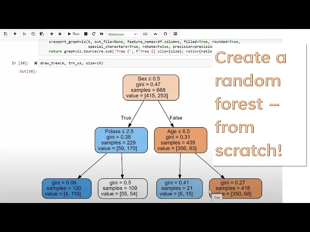
can say: please create a decision tree classifier with at most four leaf nodes. And one very nice thing it has is it can draw the tree for us. So here's a tiny little draw_tree function. And you can see here it's going to first of all split on sex, now, it looks a bit weird to say sex is less than or equal to 0.5 but remember what our binary characteristics are coded as zero or one, so that's just how we, you know, easy way to say males versus females. And then here we've got for the females,

what class are they in, and for the males what age are they. And here's our four leaf nodes. So for the females in first class 116 of them survived and four of them didn't so… very good idea to be a “well to do” woman on the Titanic. On the other hand, males adults: 68 survived 350 died so, very bad idea to be a male adult on the Titanic. So you can see you can kind of get a quick summary of what's going on and one of the reasons people tend to like decision trees, particularly for

exploratory data analysis, is it does allow us to get a quick picture of what are the key driving variables in this data set and how much do they kind of predict what was happening in the data. Okay, so it's around the same splits as us and it's got one additional piece of information we haven't seen before, this is something called “Gini”. “Gini” is just another way of measuring how good a split is, and I've put the code to calculate “Gini” here. Here's how you can think of “Gini”: How likely is it that, if you go

into that sample and grab one item and then go in again and grab another item, how likely is it that you're going to grab the same item each time. And so, if that, if the entire leaf node is just people who survived or just people who didn't survive the probability would be one, you get the same time, same every time. If it was an exactly equal mix, the probability would be 0.5. So that's why we just, yeah, that's where this formula comes from in the binary case. And in fact you can see it here, right,

this group here is pretty much 50-50 so “Gini” is 0.5. Or else this grip here is nearly 100% in one class so “Gini” is nearly zero —so that backwards is one minus. And I think I've written it backwards here as well, so… I've got to fix that. So this decision tree is, you know, we would expect it to be more accurate so we can calculate its mean absolute error. And for the “OneR”, so just doing males versus females, what was our score? Here we go, 0.407. Uh, should we have a, do we have an accuracy

score, somewhere, here we are, 0.336. Oh that was for ‘LogFare’ and for ‘Sex’ it was 0.215, okay so 0.215. So that was for the “OneR” version, for the decision tree with four leaf nodes 0.224 so it's actually a little worse, right? And I think it just reflects the fact that this is such a small data set and the “OneR” version was so good we haven't really improved it that much, or not enough to really see it amongst the randomness of such a small validation set. We could go further to 50, a minimum of 50 samples

per Leaf node. So that means that in each of these, see how it says “samples”, which in this case is passengers on the Titanic, there's at least... there's 67 people that were... were female first class Less than 28. That's how you define that. So this decision tree keeps building, keep splitting until it gets to a point where there's going to be less than 50 at which point it stops splitting that... that leaf. So you can see they're all got at least 50 samples and so here's the decision tree that builds. As you can see, it

doesn't have to be like constant depth, right? So this group here, which is males who had cheaper fares and who were older than 20 but younger than 32... yeah actually younger than 24. and actually super cheap fares and so forth right. So it keeps going down until we get to that group. So let's try that decision tree. That decision tree has an absolute error of 0.183 so not surprisingly you know once we get there it's starting to look like it's a little bit better. So there's a model and this is a Kaggle competition so therefore

we should submit it to the leaderboard. And. you know.one of the... you know... biggest mistakes I see not just beginners but every level of practitioner make on Kaggle is not to Submit to the leaderboard, spend months making some perfect thing right but you actually got to see how you're going and you should try and submit something to the leaderboard every day. So you know, regardless of how rubbish it is because you want to improve every day. So you want to keep iterating. So to submit something to the leaderboard you generally have to provide a CSV

file and so we're going to create a CSV file. And we're going to apply the category codes to get the category for each one in our test set. we're going to set the survived column to our predictions and then we're going to send that off to a CSV. And so yeah so I submitted that and I got to score a little bit worse than most of our linear models and neural nets but not terrible, you know. It was... it's... it's just doing an okay job. Now one interesting thing for the decision tree is there was

a lot less preprocessing to do, did you notice that? We didn't have to create any dummy variables for... for our categories And like, you certainly can create dummy variables but you often don't have to. So for example you know... for… for “class” you know it's... it's one two or three, you can just split on one, two, or three, you know. Even for like, what was that thing... like the... the “embarkation city code”, like we just convert them kind of arbitrarily to numbers one, two, and three, and you can split on those numbers. So with Random

Forest also... not Random Forest, not there yet... decision trees, yeah... you can generally get away with not doing stuff like dummy variables. In fact, even taking the log of “fair” we only did that to make our graph look better but if you think about it, splitting on log fare less than 2.7 is exactly the same as splitting on Fair is less than e to the 2.7 you know or whatever log base we used, I can't remember. So all that a decision tree cares about is the ordering of the data and this is another reason that

decision tree based approaches are fantastic because they don't care at all about outliers, you know... long tail distributions, categorical variables whatever. You can throw it all in and it'll do a perfectly fine job. So For tabular data I would always start by using a decision tree based approach and kind of create some baselines and so forth because it's... it's really hard to mess it up and that's important. So yeah... so here for example is “Embarked”, right? It... it was coded originally as the first letter of the city they embarked in, but we turned it into

a categorical variable and so pandas for us creates this this vocab this list of all of the possible values and if you look at the codes attribute you can see it's that S is the... zero one two... so S has become 2, C has become zero and so forth, right. So that's how we're converting the categories, the strings into numbers that we can sort and group by. So yeah... so if we wanted to split C into one group and Q and S in the other we can just do, okay, less than a quarter one point

0.5. Now of course if we wanted to split C and S into one group and Q into the other we would need two binary splits first C on one side and Q and S on the other and then Q and S into Q versus S and then the Q and S leaf nodes could get similar Predictions. So like you do have, like sometimes it can take a little bit more messing around but most of the time I find categorical variables work fine as numeric in decision tree based approaches and as I say here I tend

to use dummy variables only if there's like less than four levels. Now, what if we wanted to make this more accurate? could we grow the tree further? I mean, we could, but, you know, there's only 50 samples in these leaves, right? it's not really… you know, if I keep splitting it, the leaf nodes are going to have so little data that's not really going to make very useful predictions. Now there are limitations to how accurate a decision tree can be. So what can we do? We can do something that's actually very, I mean, I find

it amazing and fascinating, comes from a guy called Leo Breiman. And Leo Breiman came up with… came up with this idea called bagging. And here's the basic idea of bagging: let's say we've got a model that's not very good because, let's say, it's a decision tree, it's really small, we've hardly used any data for it Right, it's not very good so, it's got error, it's got errors on predictions. It's not a systematically biased error, it's not always predicting too high or always predicting too low, I mean, decision trees, you know, on average will predict the

average, right? but it has errors. So what I could do is I could build another decision tree in some slightly different way that would have different splits and it would also be not a great model, but it predicts the correct thing on average, it's not completely hopeless and again, you know, some of the errors are a bit too high and some are a bit too low. And I could keep doing this so, if I could create building lots and lots of slightly different decision trees I'm going to end up with say a hundred different models,

all of which are unbiased, all of which are better than nothing, and all of which have some errors a bit high, some bit low, whatever. So what would happen if I averaged their predictions? Assuming that the models are not correlated with each other Then you're going to end up with errors on either side of the curve: the correct prediction, some are a bit high, some are a bit low, there'll be this kind of distribution of errors, right? And the average of those errors will be zero, and so that means the average of the predictions of

these multiple uncorrelated models —each of which is unbiased— will be the correct prediction because they have an error of zero. And this is a mind-blowing insight, it says that if we can generate a whole bunch of uncorrelated, unbiased models, we can average them and get something better than any of the individual models because the average of the error will be zero. So all we need is a way to generate lots of models. Well we already have a great way to build models —which is to create a decision tree— how do we create lots of them?

how to create lots of unbiased but different models? Well, let's just grab a different subset of the data each time, let's just grab at random half the rows and build a decision tree, and then grab another half of the rows and build a decision tree, And grab another half the rows and build a decision tree. Each of those decision trees is going to be not great —it's only using half the data— but it will be unbiased, it will be predicting the average on average, it will certainly be better than nothing because it's using, you know,

some real data to try and create a real decision tree. They won't be correlated with each other because they're each random subsets. So that meets all of our criteria for bagging. When you do this you create something called a “Random Forest”. So let's create one in four lines of code. So here is a function to create a decision tree, so let's say, what —this is just the proportion of data— so let's say we put 75% of the data in each time —or we could change it to 50%— whatever, so this is the number of samples

in this subset —I call it n— and so let's at random choose n times the proportion we requested from the sample and build a decision tree from that. And so now let's, 100 times, get a tree, and stick them all in a list using a list comprehension. And now let's grab the predictions for each one of those trees and then let's stack all those predictions up together and take their mean. And that is a Random Forest. And, what do we get?, one, two, three, four, five, six, seven, eight, that's some, yeah, seven lines of code.

So Random Forests are very simple. This is a slight simplification, there's one other difference that Random Forests do which is when they build the decision tree they also randomly select a subset of columns and they select a different random subset of columns each time they do a split. And so the idea is you kind of want it to be as random as possible but also somewhat useful. So we can do that by creating a “RandomForestClassifier”, say how many trees do we want, how many samples per leaf and then fit —that is what we just did—

and here's our mean absolute error which… Yeah, again, it's like not as good as our decision tree but it's still pretty Good and again it's such a small data set it's hard to tell if that means anything and so we can submit that to Kaggle. So earlier on I created little function to submit to Kaggle, so now I just create some predictions and I submit to Kaggle. And, yeah, looks like it gave nearly identical results to a single tree. Now to one of my favorite things about Random Forest —and I should say, in… in most

real world data sets of reasonable size, Random Forest basically always give you much better results than decision trees, this is just a small data set to show you what to do. One of my favorite things about Random Forests is we can do something quite cool with it, what we can do is we can look at the underlying decision trees they create, so we've now got 100 decision trees, and we can see what columns did it find a split on and so, say here, okay well the first thing it spit on was ‘Sex’, and it improved

the Gini from 0.47 to —now just take the weighted average of 0.38 and 0.31 weighted by the samples— so that's probably going to be, I don't know, about 0.33. So I'd say, okay, it's like 0.14 Improvement in Gini thanks to ‘Sex’. And we can do that again: okay, we'll then ‘PClass’, you know, how much did that improve Gini, again, we keep weighting it by the number of samples as well. ‘LogFare’, how much does that improve Gini and we can keep track: for each column of, how much in total did they improve the Gini in this

decision tree. And then do that for every decision tree, and then add them up per column and that gives you something called a feature importance plot, and here it is. And a feature importance plot tells you how important is each feature, how often did the trees pick it and how much did it improve the Gini when it did. And so, we can see from the feature importance plot that ‘Sex’ was the most important, and class was the second most important and everything else was a long way back. And this is another reason, by the way,

why a Random Forest isn't really particularly helpful: because it's just such a easy split to do, right? basically all that matters is, You know, what class you're in and whether you're male or female. And these feature importance plots, remember: because they're built on Random Forests, and Random Forests don't care about, really, the distribution of your data and they can handle categorical variables and stuff like that, that means that you can basically, any tabular data set you have, you can just plot this, right away, and Random Forests, you know, for most data sets, only take a

few seconds to train, you know, really most of a minute or two. And so, if you've got a big data set and, you know, hundreds of columns: do this first and find the 30 columns that might matter, it's such a helpful thing to do. So I've done that, for example, I did some work in credit scoring, so we're trying to find out which things would predict who's going to default on a loan and I was given something like seven thousand columns from the database, now I put it straight into a Random Forest and found, I

think, there was about 30 columns that seemed kind of interesting. I did that like two hours after I started the job And I went to the head of marketing and the head of risk and I told them: here's the columns I think that we should focus on, and they were like: “oh my God, we just finished a two-year consulting project with one of the big consultants, paid the millions of dollars, and they came up with a subset of these… «laughs» There are other things that you can do with Random Forests along this path, I'll touch

on them briefly, and specifically I'm going to look at Chapter 8 of the book, which goes into this in a lot more detail. And particularly interestingly Chapter 8 of the book uses a much bigger and more interesting data set which is auction prices of heavy industrial equipment, I mean, it's less interesting historically but more interestingly numerically. And so, some of the things I did there on this data set — sorry this isn’t from the data set, this is from the scikit-learn documentation— they looked at how, as you increase the number of estimators, so the number

of trees, How much does the accuracy improve. So I then did the same thing on our data set, so I actually just added up to 40, more and more and more trees, and you can see that basically —as predicted by that kind of an initial bit of hand wavy theory I gave you— that you'd expect the more trees, the lower the error, because the more things you're averaging and that's exactly what we find: the accuracy improves as we have more trees. John what's up… John: Oh, Víctor… it is possible you might have just answered his

question actually as he typed it— but he's asking on the same theme: the number of trees in a Random Forest. Does increasing the number of trees always translate to a better error? Jeremy: yes it does, always, I mean: tiny bumps, right? but yeah, once you smoothed it out. But decreasing returns and… if you end up productionizing a Random Forest, then, of course, every one of these trees, you have to, you know, go through for, at inference time, So it's not that there's no cost, I mean, having said that, zipping through a binary tree is the

kind of thing you can really do fast, in fact, it's it's quite easy to like literally spit out C++ code with a bunch of if statements and compile it and get extremely fast performance. I don't often use more than 100 trees, this is a rule of thumb… is that the only one John? okay So, then there's another interesting feature of Random Forests which is: remember how in our example we trained with 75% of the data on each tree, so that means for each tree there was 25% of the data we didn't train on. Now this

actually means if you don't have much data, in some situations you can get away with not having a validation set, and the reason why is because for each tree we can pick the 25% of rows that weren't in that tree and see how accurate that tree was on those rows and we can average for each row their accuracy on all of the trees in which they were not part of the training, and that is called the Out-of-Bag Error or OOB error. And this is built in, also, scikit-learn you can ask for an OOB prediction… Uhm,

John! John: Just before we move on, Zakia has a question about bagging: so we know that bagging is powerful as an ensemble approach to machine learning, would it be advisable to try out bagging being first when approaching a particular, say, tabular task, before deep learning? So that's the first part of the question, and the second part is: could we create a bagging model which includes fast.ai deep learning models? Jeremy: Yes, absolutely. So, to be clear, you know, bagging is kind of like a meta method, it's not a prediction, it's not a method of modeling itself,

it's just a method of combining other models. So Random Forests, in particular, as a particular approach to bagging. is a, you know, I would probably always start, personally, a tabular project with a Random Forest because they're nearly impossible to mess up, and they give good insight, And they give a good base case. But yeah, your question then about “can you bag other models?” is a very interesting one, and the answer is: you absolutely can. And people very rarely do, but we will, we will, quite soon, maybe even today. So I, you know… you might be

getting the impression I'm a bit of a fan of Random Forests, and (~before I was…) before, you know, people thought of me as the Deep Learning guy, people thought of me as the Random Forest guy. I used to go on about Random Forests all the time and one of the reasons I'm so enthused about them isn't just that they're very accurate or (~that they require, you know…) that they're very hard to mess up and require very little (~processing…) pre-processing, but they give you a lot of quick and easy insight. And specifically these are the five

things which I think that we're interested in and all of which are things that random for us are good at. They will tell us how confident are we in our predictions on some particular row? So when somebody, you know… when we're giving a loan to somebody We don't necessarily just want to know “How likely are they to repay?” but we'd also like to know “How confident are we that we know?” because if we're… if we're like well we think they'll repay but we're not confident of that we would probably want to give them less of

a loan. And another thing that's very important is when we're then making a prediction… so again, for example, for credit… let's say you rejected that person's loan… “Why?...” And a Random Forest will tell us “What what is the… what is the reason that we made a prediction.” And you'll see why, and all these things. Which columns are the strongest predictors - you've already seen that one, right, that's the Feature Importance Plot. Which columns are effectively redundant with each other, i.e. they're basically highly correlated with each other. And then one of the most important ones… As

you vary a column how does it vary the predictions? So for example in your credit model, how does your prediction of risk vary as you vary… (well something that probably the regulator would want to know might Be some, you know…) some protected variable like you know race or some socio-demographic characteristics that you're not allowed to use in your model. So they might check things like that. For the first thing: “How confident are we in our predictions using a particular row of data?” There's a really simple thing we can do which is… remember how when we

calculated our predictions manually we stacked up the predictions together and took their mean? Well what if you took their standard deviation instead? So if you stack up your predictions and take their standard deviation, and if that standard deviation is high, that means all of them (all of the trees) are predicting something different!! And that suggests that we don't really know what we're doing. And so that would happen if different subsets of the data end up getting completely different trees for this particular row. So there is (like…) a really simple thing you can do to get

a sense of your prediction confidence. Okay, “Feature Importance” we've already discussed After I do feature importance (you know…) like I said when I had the (what) 7,000 or so columns I got rid of like all-but 30. That doesn't tend to improve the predictions of your Random Forest very much, if at all, but it certainly helps (like, you know…) kind of logistically thinking about cleaning up the data, you can focus on cleaning those 30 columns, and stuff like that. So I tend to remove the low importance variables. I'm going to skip over this bit about removing

redundant features because it's a little bit outside what we're talking about, but definitely check it out in the book, something called a “Dendrogram.” But what I do want to mention is the “Partial Dependence.” This is the thing which says, “What is the relationship between a column and the dependent variable - and so this is something called a “Partial Dependence Plot.” Now this one's actually not specific to Random Forests. A partial dependence plot is something you can do for basically any machine learning model. Let's first of all look at one and then talk about how we

make it. So in this dataset we're looking at the relationship… we're looking at the sale price at auction of heavy industrial equipment like bulldozers - this is specifically the blue books for bulldozers Kaggle competition. And a partial dependence plot between the year that the bulldozer -or whatever was made- and the price it was sold for (this is actually the log price) is that it goes up. More recent bulldozers… more recently made bulldozers are more expensive. And as you go back… back to older and older bulldozers, they're less and less expensive, to a point. And maybe

these ones are some classic bulldozers you pay a bit extra for. Now you might think that you could easily create this plot by simply looking at your data at each year and taking the average sale price, but that doesn't really work very well. I mean it kind of does, but it kind of doesn't. Let me give an example. It turns out that one of the biggest predictors of sale price for industrial equipment is whether it has air conditioning And so air conditioning is, you know… it's an expensive thing to add and it makes the equipment

more expensive to buy. And most things didn't have air conditioning back in the 60s and 70s and most of them do now. So if you plot the relationship between year made and price you're actually going to be seeing a whole bunch of when… you know… “How popular was air conditioning?” right, so you get this this cross-correlation going on. But we just want to know… what's just the impact of the year it was made all else being equal. So there's actually a really easy way to do that, which is: We take our data set ~(we take

the we…) and we leave it exactly as it is, so just use the training dataset… but we take every single row - and for the year made column we set it to 1950. And so then we predict for every row what would the sale price of that have been if it was made in 1950, and then we repeat it for 1951, and then repeat it for 1952 and so forth, and then we plot the averages. And that does exactly what I just said, remember I said the special words, “all else being equal…” This is setting

everything else equal. It's the… Everything else is the data as it actually occurred and we're only varying YearMade. And that's what a partial dependence plot is! That works just as well for Deep Learning or Gradient Boosting Trees or Logistic Regressions or whatever. It's a really cool thing you can do. And you can do more than one column at a time, you know… You can do two-way partial dependence plots, for example. Okay so then another one I mentioned was: “Can you describe why a particular prediction was made? So how did you decide for this particular row

to predict this particular value?” And this is actually pretty easy to do - there's a thing called Tree Interpreter but we could you could easily create this in about a half a dozen lines of code. All we do is we're saying, okay this customers come in, they've asked her a loan, we put in all of that data through the Random Forest, spat out a prediction… We can actually have a look and say okay, “Well that in Tree #1 what's the path that went down Through the tree to get to the leaf node?” And we can

say, oh well, first of all it looked at sex, and then it looked at postcode, and then it looked at income, and so we can see exactly in Tree #1 which variables were used and what was the change in ginni for each one. And then we could do the same in Tree #2, same in Tree #3, same in Tree #4… Does this sound familiar? It's basically the same as our Feature Importance Plot, right, but it's just for this one row of data. And so that will tell you basically the Feature Importances for that one particular

prediction. And so then we can plot them, like this. So for example, this is an example of an auction price prediction, and according to this plot, you know, so we predicted that the net would be… (oh, this is just a change from…) So I don't actually know what the price is, but this is how much each one impacted the price. So Year Made, I guess this must have been an older tractor - it caused our prediction of the price to go down. But then it must have been a larger machine - the Product Size caused

it to go up, a Coupler System made it go up, Model ID made it go up, and so forth, right. So you can see the Reds says this made our prediction go down. Green made our prediction go up. And so overall you can see which things had the biggest impact on the prediction and what was the direction for each one. So it's basically a feature importance plot but just ~(for a single roll) for a single row Any questions John? John: Yeah, there are a couple that have, that have sort of queued up, this is a,

this is a good spot to, to jump to them. So, first of all, Andrew is asking, jumping back to the OOB era: “would you ever exclude a tree from a forest you've had if it had a bad Out of Bag Error?” Like if you, if you have a bogus, if you had a particularly bad tree in your ensemble Jeremy: Yeah… John: Might you just drop… Would you delete a tree That was not doing its thing? It's not playing its part. Jeremy: No you wouldn't. If you start deleting trees then you are no longer having an

unbiased prediction of the dependent variable. You are biasing it by making a choice so, even the bad ones, will be improving the quality of the overall average. John: All right, thank you. Zakia followed up with the question about bagging and we're just going, you know, layers and layers here, you know: we could go on and create ensembles of bagged models? and, you know, is it reasonable to assume that they would continue… Jeremy: So that's not going to make much difference, right? If they're all like… you could take your 100 trees, split them into groups of

ten, create ten bagged ensembles and then average those but the average of an average is the same as the average. You could like have a wider range of other kinds of models, you could have like Neural Nets trained on different subsets as well but again, it's just the average of an average, we'll still give you the average. John: Right, so there's not a lot of value in, kind of, structuring the ensemble you just… Jeremy: I mean, some, some ensembles you can structure, but not bagging. Bagging's the simplest one, it's the one I mainly use, there

are more sophisticated approaches but this one is nice and easy. John: All right, and there's one that is a bit specific and it's referencing content you haven't covered but we're here now so... and it's on explainability so, feature importance of Random Forest models sometimes has different results when you compare it to other explainability techniques like SHAP, S-H-A-P, or LIME. And we haven't covered these in the course but Amir is just curious if you've got any thoughts on which is more accurate or reliable: Random Forest feature importance or other techniques Jeremy: I would lean towards, more

immediately, trusting Random Forest Feature Importances over other techniques on the whole, on the basis that it's very hard to mess up a Random Forest. So, yeah, I feel like pretty confident that a Random Forest Feature Importance is gonna be pretty reasonable as long as this is the kind of data which a Random Forest is likely to be pretty good at, you know, doing, you know, if it's like a computer vision model Random Forest aren’t particularly good at that and so, one of the things that Breiman talked about a lot was explainability and he's got a

great essay called the two cultures of statistics (“Statistical Modeling: The Two Cultures”) in which he talks about —I guess what nowadays call kind of like data scientists, machine learning folks versus classic statisticians—. And he was, you know, definitely a data scientist well before the label existed. And he pointed out, yeah, you know, first and foremost you need a model that's accurate. It needs to make good predictions. A model that makes bad predictions, will also be bad for making explanations because it doesn't actually know what's going on. So if, you know, if you, if you've got

a Deep Learning model that's far more accurate than your Random Forest then it's, you know, explainability methods from the Deep Learning model world probably be more useful because it's explaining a model that's actually correct. All right, let's take a 10 minute break and we'll come back at five past seven. Welcome back, one person pointed out I noticed I got the chapter wrong — it's Chapter 9 not Chapter 8 in the book, I guess I can't read. Somebody asked during the break about overfitting. Can you overfit a Random Forest?. Basically no, not really, adding more trees

will make it more accurate. It kind of asymptotes so you can't make it infinitely accurate by using infinite trees but certainly you know adding more trees won't make it worse. If you don't have enough trees and you let the trees grow very deep: that could overfit. So you just have to make sure you have enough trees. Radek told me about this experiment he did during… Radek talked to me during the break about an experiment he did, which is something I've done something similar, which is adding Lots and lots of randomly generated columns to a data

set and try to break the Random Forest. And if you tried it, it basically doesn't work, it's like, it's really hard to confuse a Random Forest by giving it lots of meaningless data, it does an amazingly good job of picking out the useful stuff. As I said, you know, I had 30 useful columns out of 7,000 and it found them perfectly well. And often, you know, when you find those 30 columns, you know, you could go to, you know —I was doing consulting at the time— go back to the client and say like: tell me

more about these columns, and say like: “oh! well that one there we've actually got a better version of that now, there's a new system, you know, we should grab that… and, oh, this column actually that was because of this thing that happened last year but we don't do it anymore…” or, you know, like you can really have this kind of discussion about the stuff you've zoomed into. You know, there are other things that you have to think about with lots of kinds of models like, particularly regression models; things like interactions. You don't have to worry

about that with Random Forests like, because you split on one column and then split on another column you get interactions for free as well. Normalization you don't have to worry about, you know you don't have to have normally distributed columns. So yeah, definitely worth a try. Now something I haven't gone into… is Gradient Boosting. But if you go to explain.ai, you'll see that my friend Terence and I have a three-part series about Gradient Boosting, including pictures of golf made by Terence. But to explain Gradient Boosting is a lot like Random Forests but rather than fitting

a tree again and again and again on different random subsets of the data… instead, what we do is we fit very, very, very small trees, so hardly ever any splits and we then say: “okay, what's the error”. So, you know, so, imagine the simplest tree would be our “OneR” raw tree of male versus female, say, and then you take what's called the residual: That's the difference between the prediction and the actual, it's the error. And then you create another tree, which attempts to predict that —a very small tree— and then you create another very small

tree which tries to predict the error from that and so forth, right? Each one is predicting the residual from all of the previous ones. And so then to calculate a prediction, rather than taking the average of all the trees, you take the sum of all the trees, because each one is predicting the difference between the actual and all of the previous trees. And that's called boosting —versus bagging— so boosting and bagging are two kind of meta ensembling techniques, and when bagging is applied to trees it's called a Random Forest and when boosting is applied to

trees it's called a Gradient Boosting Machine or Gradient Boosted Decision Trees. Gradient Boosting is, generally speaking, more accurate than Random Forests, but you can absolutely overfit and so therefore it's not necessarily my first go-to thing. Having said that there are ways to avoid overfitting, but yeah, (it's just, it's not, You know) because it's breakable, it's not my first choice. But yeah, check out our stuff here if you're interested and, you know, there is stuff which largely automates the process, there's lots of hyper parameters you have to select. People generally just, you know, try every combination

of hyper parameters and, in the end, you generally should be able to get a more accurate Gradient Boosting model than Random Forest… but not necessarily by much. Okay, so that was the Kaggle notebook on Random Forests: “How random forests really work”. So, what we've been doing is having this daily walk-through where me and —I don't know how many— 20 or 30 folks get together on a Zoom call and chat about, you know, getting through the course, and setting up machines, and stuff like that. And, you know, we've been trying to kind of practice what, you

know, things along the way and so, a couple of weeks ago, I wanted to show: What does it look like to pick a Kaggle competition and just like do the normal, sensible, kind of mechanical steps that you would do for any computer vision model. And so the competition I picked was Paddy Disease Classification, which is about recognizing diseases, rice diseases and rice paddies. And yeah I spent —I don't know— a couple of hours, or three —I can't remember—. A few hours, throwing together something and I found that I was number one on the leaderboard and

I thought: “oh, that's interesting”, like, because you never quite have a sense of how well these things work. And then I thought: “well there's all these other things we should be doing as well”, and I tried three more things, and each time I tried another thing, I got further ahead at the top of the leaderboard. So I thought it'd be cool to take you through the process. I'm going to do it reasonably quickly because the walkthroughs are all available for you to see the entire thing in, you know, seven hours of detail —or however long

we probably were, six to seven hours of conversations— But I want to kind of take you through the basic process that I went through. So since I've been studied to do more stuff on Kaggle, you know, I realized there's some kind of manual steps I have to do each time, particularly because I like to run stuff on my own machine and then kind of upload it to Kaggle. So to do, to to make my life easier I created a little module called fastKaggle which you'll see in my notebooks from now on, which you can download

from pip or conda, and as you'll see it makes some things a bit easier. For example: downloading the data for the Paddy Disease Classification, if you just run “setup_comp()” and pass in the name of the competition, if you are on Kaggle, it will return a path to that competition data that's already on Kaggle; if you are not on Kaggle and you haven't downloaded it, it will download and unzip the data for you. If you're not on Kaggle and you have downloaded and unzip the data, it will return a path to the one that you've already

downloaded. Also if you are on Kaggle You can ask it to make sure that pip things are installed —that might not be up to date otherwise— so that's basically one line of code now gets us all set up and ready to go. So this path… so I ran this particular one on my own machine, so it downloaded and unzipped the data. I've also got links to the six walkthrus so far: these are the videos. Oh yes, and here's my result after these four attempts, that's a few fiddling around at the start. So the overall approach

at, is, well and this is not just a Kaggle competition, right? the reason I like looking at Kaggle competitions is you can't hide from the truth in a Kaggle competition, you know, when you're working on some work project or something, you might be able to convince yourself and everybody around you that you've done a fantastic job of not overfitting, and that your model's better than what anybody else could have made, and whatever else; but the brutal assessment of the private leaderboard will tell you the truth. Is your model actually predicting things correctly? and, is it

overfit? Until you've been through that process, you know, you're never going to know. And a lot of people don't go through that process because at some level they don't want to know. But it's okay, you know, nobody needs it, you don't have to put your own name there. I always did, right from the very first one I wanted, you know, if I was going to screw up royally I wanted to have the pressure on myself of people seeing me in last place. But you know, it's fine, you can do it all anonymously and you'll actually

find as you improve you'll have so much self-confidence, you know. And the stuff we do in a Kaggle competition is indeed a subset of the things we need to do in real life, but it's an important subset, you know. Building a model that actually predicts things correctly and doesn't overfit is important. And furthermore structuring your code and analysis in such a way that you can keep improving over a three-month period without gradually getting into more and more of a tangled mess of impossible to understand code and having no idea what UntitledCopy13 was, And why it

was better than 25, right, this is all stuff you want to be practicing, ideally well away from customers or whatever, you know, before you've kind of figured things out. So the things I talk about here about doing things well in this Kaggle competition should work, you know, in other settings as well. And so these are the two focuses that I recommend: Get a really good validation set together - we've talked about that before, right, and in a Kaggle competition (that's like…) it's very rare to see people do well in a Kaggle competition who don't have

a good validation set. Sometimes that's easy, and this competition actually it is easy, because the the the test set seems to be a random sample, but most of the time it's not actually, I would say. And then how quickly can you iterate? How quickly can you try things and find out what worked? So obviously you need a good validation set otherwise it's impossible to iterate. And so “quickly iterating” means not saying what is the biggest, you know, OpenAI takes four months on 100 TPUs model that I can train. It's what can I do that's going

to train in a minute or so and will quickly give me a sense of… like well I could try this, I could try that, what things going to work, and then try, you know, 80 things. It also doesn't mean that saying like… Oh I heard this is amazing new Bayesian hyper parameter tuning approach, I'm going to spend three months implementing that, because that's gonna, like, give you one thing. But actually to do well in these competitions or in machine learning in general, you actually have to do everything reasonably well. And doing just one thing really

well will still put you somewhere about last place. So I actually saw that a couple of years ago, an Aussie guy who's a very very distinguished machine learning practitioner, actually put together a team and entered a Kaggle competition and literally came in last place, because they spent the entire three months trying to build this amazing new fancy thing and never actually, never actually iterated. If you iterate I guarantee you won't be in last place. Okay, so here's how we can grab our data, With FastKaggle, and it gives us (tells us) what path it's in. And

then I set my random seed - and I only do this because I'm creating a notebook to share. You know, when I share a notebook I like to be able to say “as you can see this is 0.83 blah blah blah right and know that when you see it, it'll be 0.83 as well. But when I'm doing stuff otherwise, I would never set a random seed. I want to be able to run things multiple times and see how much it changes each time, all right, because that'll give me a sense of like… are the modifications

I'm making, changing it because they're improving it or making it worse, or is it just random variation. So if you (or if you) always set a random seed, that's a bad idea because you won't be able to see the random variation. So this is just here for presenting a notebook. Okay, so the data they've given us, as usual, they've got a sample submission, they've got some test set images, they've got some training set images, a CSV file about the training set and then these other two you can ignore because I created them. So let's grab

a path to train images… and so do you remember get_image_files()... so that gets us a list of the file names of all the images here recursively, so we could just grab the first one, and take a look - so it's 480 by 640. Now we've got to be careful. This is a pillow image (Python Imaging Library image.) In the imaging world they generally say columns by rows. In the array slash tensor world we always say rows by columns. So if you ask pytorch what the size of this is it'll say 640 by 480, and I

guarantee at some point this is going to bite you. So try to recognize it now. Okay so they're kind of taller than they are… at least this one is taller than it is wide. So I actually like to know were they all this size, because it's really helpful if they all are all the same size, or at least similar. Believe it or not the amount of time it takes to decode a JPEG is actually quite significant and so figuring out what size these things are is actually going to be pretty slow, But my fastcore library

has a parallel sub module which can basically do anything that you can do in Python, it can do it in parallel. So in this case we wanted to create a pillow image and get its size. So if we create a function that does that and pass it to parallel, passing in the function and the list of files, it does it in parallel and that actually runs pretty fast. And so here is the answer… (I don't know how this happened…) 10,403 images are indeed 480 by 640 and four of them aren't. So basically what this says

to me is that we should pre-process them or you know at some point process them so that they're probably all 480 by 640, or all basically kind of the same size. We'll pretend they're all this size but we can't not do some initial resizing otherwise this is going to screw things up. So like the probably the easiest way to do things, the most common way to do things, is to either squish or crop every image to be a square. So squishing is when you just… (in this case…) squish the aspect ratio down as Opposed to

cropping randomly a section out. So if we call Resize() ‘squish’ it will squish it down, and so this is 480 by 480 squared. So this is what it's going to do to all of the images first, on the CPU, that allows them to be all batched together into a single mini batch (everything in a mini batch has to be the same shape otherwise the GPU won't like it,) and then that many batches put through data augmentation, and it will grab a random subset of the image, and make it a 128 by 128 pixels. And here's

what that looks like, here's our data. So show_batch() works for pretty much everything, not just in the fast AI library, but even for things like FastAudio which are kind of community based things. You should better use show_batch() on anything and see, or hear, or whatever, what your data looks like. I don't know anything about rice disease but apparently these are various rice diseases and this is what they look like. So I jump into creating models much more quickly than most people, because I find… model, you know, Models… are a great way to understand my data,

as we've seen before. So I basically build a model as soon as I can, and I want to create a model that's going to let me iterate quickly. So that means that I'm going to need a model that can train quickly. So Thomas Capell and I recently did this big project “The Best Vision Models For Fine Tuning” where we looked at nearly a hundred different architectures from Ross Whiteman's Timm Library (Pytorch Image Model Library) and looked at which ones could we fine-tune - which ones had the best transfer learning results. And we tried two different

datasets, very different datasets. One is the pets dataset that we've seen before - so trying to predict what breed of pet is from 37 different breeds. And the other was a satellite imagery data set called planet. So very very different data sets in terms of what they contain and also very different sizes. The planet one is a lot smaller the Pets one is a lot bigger. And so the main things we measured were how much memory did it use, how accurate was it, and how long did it take to fit. And then I created this

score which can… which combines the fit, time and error rate together. And so this is a really useful table for picking a model. And now in this case I want to pick something that's really fast, and there's one clear winner on speed, which is resnet26d. And so its accuracy was 6% versus the best was like 4.1% - so okay it's not amazingly accurate, but it's still pretty good, and it's going to be really fast, so that's why I picked “resnet26d. A lot of people think that when they do deep learning they're going to spend all

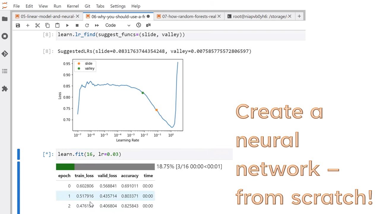
of their time learning about exactly how a resnet26d is made and convolutions and resonant blocks and transformers and blah blah blah. We will cover all that stuff in Part Two and a little bit of it next week but it almost never matters, right, it's just a function, right, and what matters is the inputs to it, and the outputs to it, and how fast it is, and how accurate it is. So let's create a learner which with a resnet26d from our data loaders, and let's run lr_find(). So lr_find() will put through one mini-batch at a time

starting at a Very very very low learning rate, and gradually increase the learning rate, and track the loss. And initially the loss won't improve because the learning rate is so small it doesn't really do anything, and at some point the learning rate is high enough that the loss will start coming down, and then at some other point the learning rate is so high that it's going to start jumping past the answer and it's going to predict worse. And so somewhere around here is a learning rate we'd want to pick. We've got a couple of different

ways of making suggestions. I generally ignore them because these suggestions are specifically designed to be conservative. They're a bit lower than perhaps optimal, in order to make sure we don't recommend something that totally screws up, but I kind of like to say, like well… How far right can I go and still see it, like, clearly really improving quickly, and so I'd pick somewhere around 0.01 for this. So I can now fine-tune our model with a learning rate of 0.01, three epochs, so look!... the whole thing took a minute! That's what we want, right, we want

to Be able to iterate, rapidly, just a minute or so. So that's enough time for me to go and you know, grab a glass of water, or do some reading, like I’m not going to get too distracted. And what did we do before we submit? Nothing! We submit as soon as we can. Okay, let's get our submission in. So we've got a model, let's get it in. So we read in our CSV file of the sample submission and so the CSV file basically looks like we're going to have to have a list of the image

file names, in order, and then a column of labels. So we can grab all the image files in the test image —like so— and we can sort them. And so now we want is —what we want is— a dataloader, which is exactly like the dataloader we use to train the model, except pointing at the test set, we want to use exactly the same transformations so there's actually a dls.test_dl() method —which does that— you just pass in the new set of items, so the test set files. So this is a dataloader which we can use for

our test set. A test dataloader has a key difference To a normal data loader which is that it does not have any labels. So that's a key distinction. So we can get the predictions for our learner, passing in that dataloader and in the case of a classification problem you can also ask for them to be decoded, decoded means rather than just get returned the probability of every rice disease for every class, it'll tell you what is the index of the most probable rice disease, that's what decoded means. So this is returning the probabilities, targets —which

obviously will be empty because it's a test set, so throw them away— and those decoded indexes which look like this: numbers from naught (0) to nine (9) because there's ten possible rice diseases. The Kaggle submission does not expect numbers naught (0) to nine (9), it expects to see strings like these. So, what do those numbers from naught (0) to nine (9) represent? We can look up our vocab to get a list, so that's zero, that's one, et cetera, that's nine. So, I realized later this is a slightly inefficient way to do it, But it does

the job I need to be able to map these to strings so, if I enumerate the vocab, that gives me pairs of numbers; zero (0): bacterial leaf blight, one (1): bacterial leaf streak, etc. I can then create a dictionary out of that, and then I can use pandas to look up each thing in a dictionary: they call that map. If you're a pandas user you've probably seen map used before being passed a function —which is really, really slow— but if you pass map a dict it's actually really, really fast, so do it this way if

you can. So here's our predictions, so we've got our submission sample: submission file “ss”, so if we replace this column label with our predictions —like so— then we can turn that into a CSV, and remember, this means, this means: run a bash command —a shell command—, head is the first few rows —let's just take a look. That looks reasonable! So we can now submit that to Kaggle. Now, iterating rapidly means everything needs to be Fast and easy. Things that are slow and hard don't just take up your time but they take up your mental energy,

so even submitting to Kaggle needs to be fast. So I put it into a cell, so I can just run this cell: api.competition_submit_cli(), this CSV file, give it a description, so just run the cell and it submits to Kaggle. And as you can see it says: here we go!, “successfully submitted”. So that submission was terrible: top eighty percent also known as bottom twenty percent, which is not too surprising, right?, I mean, it's one minute of training time. But it's something that we can start with and that would be like: however long it takes to get

to this point, that you put in our submission, now you've really started, right? because then tomorrow you can try to make a slightly better one. So I'd like to share my notebooks and so, even sharing the notebook, I've automated. So part of fastkaggle is: you can use this thing called push_notebook and that sends it off to Kaggle to create… A notebook on Kaggle, there it is, and there's my score. As you can see it's exactly the same thing. Why would you create public notebooks on Kaggle? Well, it's the same brutality of feedback that you get

for entering a competition, but this time rather than finding out, in no uncertain terms, whether you can predict things accurately; this time you can find out —no it's no uncertain terms— whether you can communicate things in the way that people find interesting and useful. And if you get zero votes, you know, so be it, right? that's something to know and then, you know, ideally go and ask some friends, like: what do you think I could do to improve? and if they say: oh, nothing, it's fantastic! you can tell: no, that's not true, I didn't get

any votes, I'll try again, this isn't good, how do I make it better, you know, and you can try and improve because if you can create models that predict things well, and you can communicate your results in a way that is clear and compelling, You're a pretty good data scientist, you know, like they're two pretty important things and so here's a great way to test yourself out on those things and improve. Yes John. John: yes Jeremy we have a sort of —I think— a timely question here from Zakia about your iterative approach. And they're asking:

“do you create different Kaggle notebooks for each model that you try?” Jeremy: yeah… John: so one Kaggle book for the first one, then separate notebooks subsequently, or do you, do append to the bottom of us — Jeremy: yeah, yeah — but what's your strategy? Jeremy: that's a great question. And I know Zaki is going through the daily walkthroughs but isn't quite caught up yet so, I would say: keep it up because in the six hours of going through this you'll see me create all the notebooks… But, if I go to the actual directory I used,

you can see them. So basically: yeah. I started with, you know, what you just saw, a bit messier without the pros, but that same basic thing, I then duplicated it to create the next one —which is here— and because I duplicated it, you know, this stuff which I still need it's still there, right? and so I run it. And I don't always know what I'm doing, you know, and so, at first, if I don't really know what I'm doing next I'm going to duplicate it, it will be called, you know, “first steps in the road

to the top part one dash copy one”, you know, and that's okay. As soon as I can I'll try to rename that, once I know what I'm doing, you know, or if it doesn't seem to go anywhere I'll rename it into something like, you know, experiment blah blah blah and I'll put some notes at the bottom and I might put it into a failed folder or something. But yeah, it's like, it's a very low tech approach that I find works really well: which is just duplicating notebooks and editing them and naming them carefully and putting

them in order And, you know, put the file name in when you submit as well. And then of course also if you've got things in git, you know, you can have a link to the git commit so you'll know exactly what it is… generally speaking from me, you know, my notebooks will only have one submission in and then I'll move on and create a new notebook so I don't really worry about versioning so much, but you can do that as well if that helps you. Yeah, so that's basically what I do and and I've worked

with a lot of people who use much more sophisticated and complex processes and tools and stuff but none of them seem to be able to stay as well organized as I am, I think they kind of get a bit lost in their tools, sometimes. And file systems and file names I think are good. John: oh great thanks so, away from that kind of dev process, more towards the specifics of, you know, finding the best model and all that sort of stuff. We've got a couple of questions that are in the same space, which is, you

know, we've got some people here talking about AutoML Frameworks which you might want to, you know, touch on for people who haven't heard of those. If you've got any particular AutoML Frameworks you think are worth recommending. Or just, more generally, how do you go trying different models. Random Forest, Gradient Boosting, Neural Networks… it just so in that space if you can comment it Jeremy: sure. I use AutoML less than anybody I know, I would guess, which is to say: never. Hyper parameter optimization: never. And the reason why is I like being highly intentional, you know,

I like to think more like a scientist and have hypotheses and test them carefully and come up with conclusions —which then I implement, you know—. So for example, in this “best vision models for fine tuning” I didn't try a huge “grid search” of every possible model, every possible learning rate, every possible pre-processing approach blah blah blah right. Instead, step one was to find out: well, which things matter, right? So, for example, “does whether we squish or crop make a difference?” you know, “are some models better With squish and some models better with crop?” and so

we just chested that for… and again, not for every possible architecture but for one or two versions of each of the main families, that took: 20 minutes. And the answer was: no, in every single case the same thing was better. So we don't need to do a grid search over that anymore, you know. Or another classic one is like, learning rates, most people do a, kind of, grid search over learning rates or they'll train a thousand models, you know, with different learning rates. But this fantastic researcher named Leslie Smith invented the learning rate finder a

few years ago, we implemented it, I think, within days of it (first) coming out as a technical report, and that's what I've used ever since: it works well and runs in a minute or so. Yeah, I mean, then like Neural Nets versus GBMs versus Random Forests, I mean, that's… that shouldn't be too much of a question on the whole, like: they have pretty clear places that they go. Like, if I'm doing computer vision I'm obviously going to use a Computer vision Deep Learning model and which one I would use, well, if I'm transfer learning —which

hopefully is, always— I would look up the two tables here: this is my table for pets which is, which are the best at fine tuning to very similar things to what they're pre-trained on, and then the same thing for planet is: “which ones are best for fine tuning for two data sets that are very different on what they're trained on”? And it happens in both case they're very similar, in particular “convnext” is right up towards the top in both cases, so I just like to have these rules of thumb and… yeah, my rule of thumb

for tabular is: Random Forest is going to be the fastest easiest way to get a pretty good result, GBMs probably going to give me a slightly better result if I need it, and can be bothered fussing around GBM I would probably, yeah, actually I probably would run a hyper parameter sweep because it is fiddly and it's fast, so you may as well. So, yeah, you know, we were able to make a slightly better submission, A slightly better model. And so, I had a couple of thoughts about this. The first thing was: that thing trained in

a minute on my home computer and then, when I uploaded it to Kaggle, it took about four minutes per epoch —which was horrifying—. And, Kaggle GPUs are not amazing but they're not that bad so I knew something was up, and what was up is I realized that they only have two virtual CPUs which nowadays is tiny, like, you know, you generally want —as a rule of thumb— about eight physical CPUs per GPU. And so, spending all of its time just reading the damn data. Now, the data was 640 by 480 and we were ending up

with only 128 pixel size bits for speed. So there's no point doing that every epoch so, step one was to make my Kaggle iteration faster, as well, and so a very simple thing to do: resize the images, so fastai has a function called resize_images() and you say: “okay, take all the train images and stick them in the destination, making them this size recursively”, and that will recreate the same folder structure over here. And so that's why I call this the training path: because this is now my training data and so, when I then, trained on

that, on Kaggle, it went down to four times faster with no loss of accuracy so, that was kind of step one was: to actually get my first iteration working. Now, still, I bet it's a long time and on Kaggle you can actually see this little graph showing: how much the CPU is being used, how much the GPU is being used; on your own home machine you can —there are tools free GPU— you know, free tools to do the same thing. I saw that the GPU was still hardly being used so it's still CPU was being

driven pretty hard, I wanted to use a better model anyway —to move up the leaderboard— so I moved from a… Oh, by the way, this graph is very useful, so this is… this is speed versus error rate by family. And so we're about to be looking at these convnext models so we're going to be looking at this one convnext_tiny… Here it is convnext_tiny. So we were looking at resnet26d, which took this long on this data set, But this one here is nearly the best (I think it's third best) but it's still very fast, and so

it's the best overall score. So let's use this, particularly because, you know, we're still spending all of our time waiting for the CPU anyway. So it turned out that when I switched my architecture to convnext it basically ran just as fast, on Kaggle, so we can then train that. Let me switch to the Kaggle version because my outputs are missing for some reason. So yeah… so I started out by running the resnet26d on the resized images and got similar error rate, but I ran a few more epochs, got 12% error rate. And so then I

do exactly the same thing but with convnext_small and 4.5% error rate, so I don't think that different architectures are just tiny little differences - this is over twice as good. And a lot of folks you talk to will never have heard of this convnext because it's very new and I've noticed a lot of people tend not to keep up to date with new things. They kind of learn something at University and then they stop… stop learning. So if somebody's still just using resnets all the time, you know, You can tell them, we've actually… we've moved

on, you know. Resnets is still probably the fastest but for the mix of speed and performance, you know, not so much. Convnext, you know again, you want these rules of thumb, right. If you're not sure what to do, this convnext, okay, and then like most things there's different sizes - there's a tiny, there's a small, there's a base, there's a large, there's an extra large, and you know it's just… well let's look at the picture. This is it here, right, large takes longer but lower error, tiny takes less time but higher error, right, so you

pick about your speed versus accuracy trade-off, for you. So for us small is great. And so yeah now we've got a 4.5% error, that's terrific! Now let's iterate! On Kaggle this is taking about a minute per epoch. On my computer it's probably taking about 20 seconds per epoch, so not too bad. So you know, one thing we could try is instead of using squish as our pre-processing, let's try using crop. So that will randomly crop out an area, and that's the default, So if I remove the “method=squish” that will crop. So you see how I've

tried to get everything into a single function, right, the single function. I can tell it… (let's go and find the definition…) what architecture do I want to train, how do I want to transform the items, how do I want to transform the batches, and how many epochs do I want to do - that's basically it, right. So this time I want to use the same architecture convnext, I want to resize without cropping, and then use the same data augmentation, and okay, error rate's about the same. So not particularly… it's a tiny bit worse, but not

enough to be interesting. Instead of cropping, we can pad. Now padding is interesting… do you see how these are all square, right, but they've got black borders… so padding is interesting because it's the only way of pre-processing images which doesn't distort them and doesn't lose anything. If you crop, you lose things. If you squish, you distort things. This does neither. Now of course the downside is that there's pixels that are literally Pointless - they contain zeros. So every way of getting this working has its compromises but this approach of resizing where we pad with zeros

is not used enough - and it can actually often work quite well - in this case it was about as good as our best so far, but no, not huge differences yet. What else could we do? Well, what we could do is… see these pictures? This is all the same picture but it's gone through our data augmentation, so sometimes it's a bit darker, sometimes it's flipped horizontally, sometimes it's slightly rotated, sometimes it's slightly warped, sometimes it's zooming into a slightly different section, but this is all the same picture. Maybe our model would like some of

these versions better than others, so what we can do is we can pass all of these to our model, get predictions for all of them, and take the average, right. So it's our own kind of like little mini-bagging approach, and this is called Test Time Augmentation. Fast.ai is very unusual in making that available in a single method. You just Pass TTA and it will pass multiple augmented versions of the image and average them for you. And so this is the same model as before, which had a 4.5%, so if instead if we get TTA predictions

and then get the error rate, wait why does it say 4.8?... last time I did this it was way better. Well that's messing things up isn't it? So when I did this originally on my home computer it went from like 4.5 to 3.9, so possibly I got a very bad luck this time. So this is the first time I've actually ever seen TTA give a worst result. So that's very weird. I wonder if it's… if I should use something other than the crop-n-padding. All right, I'll have to check that out, and I'll try and come

back to you and find out why in this case this one was worse. Anyway take my word for it every other time I've tried it TTA has been better, so then you know now that we've got a pretty good way of resizing, we've got TTA, we've got a good training process, let's just make bigger images, and something that's really interesting and a lot of people Don't realize is your images don't have to be square, they just all have to be the same size, and given that nearly all of our images are 640x480 we can just

pick, you know, that aspect ratio (so for example 256x192) and we'll resize everything to the same aspect ratio rectangular, and that should work even better still. So if we do that we'll do 12 epochs… okay now our error rate is down to 2.2% And then we'll do TTA. Okay this time you can see it actually improving, down to under 2% so that's pretty cool, right… we've got our error rate… at the start of this notebook we were at 12% and by the time we've got through our little experiments we're down to under 2%. And nothing

about this is in any way specific to rice, or this competition, you know, it's like this is a very mechanistic, you know, standardized approach, which you can use for certainly any kind of this type of computer vision competition - they'd have computer vision data set almost. But you know, it Looked very similar for a collaborative filtering model, a tabular model, NLP model, whatever. So, of course, again, I want to submit as soon as I can. So, just copy and paste the exact same steps I took last time basically for creating a submission. So, as I

said last time, we did it using pandas, but there's actually an easier way. So the step where here I've got the numbers from naught to nine, which is like, which… which rice disease is it? so here's a cute idea; we can take our vocab, and make it an array so that's going to be a list of 10 things and then we can index into that vocab with our indices which is kind of weird this is a list of 10 things this is a list of… I don't know four or five thousand things? so this will

give me four or five thousand results which is each vocab item for that thing? So this is another way of doing the same mapping, and I would spend time playing with this code to understand what it does, because it's the kind of like very fast, what, you know, not just in terms of writing, but this this… the… this would optimize… you know on on The CPU very very well.This is the kind of coding you want to get used to, this kind of indexing. Anyway, so then we can submit it just like last time, and when

I did that I got in the top 25 percent, and that's… that's where you want to be, right? Like generally speaking, I find in Kaggle competitions the top 25 percent is like, you're kind of like solid competent level? you know? look it's not to say like, it's not easy you've got to know what you're doing, but if you get in the top 25, and I think you can really feel like yeah this is… this is a… you know very reasonable attempt, and so that's I think, this is a very reasonable attempt. Okay before we wrap

up, John any last questions? John: Um yeah, there's there's two I think that would be good if we could touch on quickly before you wrap up; one from Victor asking about TTA: “when I use TTA during my training process do I need to do something special during inference or is this something you use only during validate?” Jeremy: Okay so just to explain TTA means “test time augmentation” so, specifically it Means inference. I think you mean augmentation during training? so yeah… so during training, you basically always do augmentation which means you're varying each image slightly so

that the model never sees the same image exactly the same twice, and so it can't memorize it. On Fast Ai – and as I say I don't think anybody else does this as far as I know – if you call TTA, it will use the exact same augmentation approach on whatever data set you pass it, and average out the prediction, but… but like multiple times on the same image, and will average them out, so you don't have to do anything different, but if you didn't have any data augmentation in training you can't use TTA. It

uses the same… by default the same data augmentation you use for training. John: Great! thank you! and the other one is about how you know when you first started this example you squared the models and you the images rather, and you talked about squashing versus cropping versus you know, clipping and scaling, and so on, but then you went on to say that these models can actually take rectangular inputs right? So there's a question that's kind of probing at that… you know, if the…” if the models can take rectangular inputs why would you ever even care

as long as they're all the same size?” Jeremy: So, I find most of the time data sets tend to have a wide variety of input sizes and aspect ratios, so you know if there's just as many tall skinny ones as wide short ones you know you doesn't make sense to create a rectangle because some of them… you're going to really destroy them, so a square is the kind of best compromise in some ways there are better things we can do which we don't have any off-the-shelf Library support for yet, and I don't think… I don't

know, that anybody else has even published about this, but we've experimented with kind of trying to batch things that are similar aspect ratios together, and use the kind of median rectangle for those and have had some good results with that, but honestly not 89, 99 percent of people, given a wide variety of aspect ratios, chuck everything into a square. John: A follow-up! this is my own interest, “have you ever looked at You know so the issue with with padding as you say is that you're putting you know black pixels there those are not NANs, those

are black pixels, that's right, and so there's something problematic to me you know conceptually about that, you know, when you… when you see for example four to three aspect ratio footage presented for broadcast on 16 to nine you get the kind of the Blurred stretch? that kind of stuff? Jeremy: No, we played with that a lot yeah? I used to be really into it actually, and fastai, still by default uses a reflection padding which means if this is… I don't know, let's say this is a 20 pixel wide thing it takes the 20 pixels next

to it and flips it over and sticks it here and it looks pretty good you know another one is copy which simply takes the outside pixel and it's a bit more like TV you know um…you know, much too much. Again, it turns out none of them really helped! plus, you know, if anything they make it worse, because in the end the computer wants to know “no this is the end of the Image there's nothing else here”, and if you reflect it for example, then you're kind of creating weird spikes that didn't exist, and the computer's

got to be like, “oh I wonder what that spike is?”, so yeah it's a great question, and I obviously spent like a couple of years assuming that we should be doing things that look more image like, but actually the computer likes things to be presented to it in as straightforward a way as possible. All right! thanks everybody! and hope to see some of you in the walkthroughs, and otherwise see you next time!