okay in this part we'll discuss dprl algorithms to address the distribution shift problem that we looked at uh in the in the last part so the broad idea towards addressing distribution shift is to be pessimistic and we look at what that means so we are so in this uh in this section what we will do is we will be in the context of acquiring methods where the q function is trained with it with an objective that tries to make it as close as possible to the expected uh to the target value computed using the reward
function plus the expected target q value under the under the policy wi-fi and the policy wi-fi is updated towards maximizing the q value which is shown in the black part of the second line what these pessimistic methods do at an abstract level is that these methods apply a penalty uh or a constraint on the policy that is shown in red that prevents the policy wi-fi to be very different from the behavior policy pi beta such a constraint is known as a policy constraint so what we do now is the policy wi-fi is not just trying
to optimize the q function meaning that it does not try to just optimize the rl objective but instead it also tries to be close to the the behavior distribution of the behavior policy pi beta what does this do really so let's look back at the at the at the q function profile that we looked at earlier by understanding what the problem is let's look at what this kind of a policy constraint would do in this example so just just to recall the q function at a particular state is shown here as a function of the
action and the behavioral policy pi beta which is marked as the dashed red line in the plot which is labeled as beta in the plot and the issue really was that outer distribution actions are unseen actions in which which are erroneously optimistic were being used for the q function backup with the policy constraint now where the policy pi 5 is constrained to be in some sense close to pi beta what is happening now is our target q function or our q s prime a prime is only being queried on actions a prime which are in
a sense uh close to the behavior policy or close to beta so those actions which are farther away and the q function values are enormously optimistic those actions will never be will not be used anymore for the q function backup so what we are doing now is we are preventing auto distribution action values to be used for the backup and this ensures that all the values that you are using during training are also themselves trained because recall from the from the from the previous slides that we are training the q function on state action pairs
drawn from the from the data set which are drawn from the behavior policy indeed and now what we're doing is we're also making sure that the target values are computed using these actions so in a sense whatever we whatever actions we are training on or whatever actions we are using to compute the regression target for the q function are also the actions on which we trained the q function so what are so what would be some practical methods or how could can we instantiate this abstract framework of policy constraints into a practical dpiral method that
you could actually implement and actually see uh performing well so in this policy constraint uh set of methods the the real choice uh here is the choice of the divergence t so pi beta is the behavior policy which we know wi-fi is the learned policy that we're learning but the choice of divergence d or this notion of metric of or or this notion of closeness is in a sense up to us so there are several ways of choosing this divergency and these methods can broadly be grouped into these uh into these four categories which will
go with uh the support matching category distribution matching category state marginal constraint category as well as implicit or closed form constraints so by looking at them that's it's beneficial to have this picture here which is essentially the old picture from before for the cube profile but it also marks what these different constraints would do schematically on this figure so let's start with support matching so support matching is an objective where what you want to do is you want to make sure that the the policy that you're learning that is wi-fi chooses actions that are in
the support of the behavior distribution meaning that the actions that it chooses should be highly or should be should be like likely enough under the behavior policy the the probability with which the the the policy chooses those actions or the the probability with which pi fi chooses an action a that is likely under pi beta may be varying and that could be either small or large as shown in one of the yellow curves in the in the in the second part of the figure however it should choose those actions to not choose anything outside such
a constraint is known as a support constraint because what it really cares for is it does not care about the density of phi phi of a given s and pi beta of a given s what it really cares about is just the fact that the action support set should be the same or should be should be our action support set for pi fi should be contained within the action support set for pi beta an example such a constraint is the mmd distance or the maximum mean discrepancy distance which approximately gives us this behavior the second
form of constraints is distribution matching which is uh which is basically the class of constraints which we typically use or probabilistic distances that we typically use like the kn divergence the total variation divergence etc and what these distances would do is uh they would try to make sure that the distribution pi phi of a given s is close to the distribution pi beta of a given s and that will give you some behavior like the one shown on the left part of the figure where one of the purple policies are feasible policies for pi phi
because they they are kind of close and pi close to pi beta in the in the density function space so density function as a whole should be closed towards tensorflow function of pi beta and like the support constraint where the density function need not be close except that the support set needs to be contained in the support side of the behavior policy there are also other alternatives like uh state marginal constraints where or state action marginal constraints where you can when instead of constraining the instead of just constraining the a given s distribution meaning that
instead of just constraining pi phi of a given s to be close to pi b of a given s you can also constrain the the the marginal state action distribution of pi phi against the marginal state action distribution of pi beta and finally there are also methods that uh sort of implement the distribution matching constraints like the kl etcetera in closed form so often what happens is that in deep learning solving constrained optimization problems can be somewhat hard sometimes so what if you already solve the constrained optimization problem for the policy constraint in closed form
and directly implemented that policy update in in in our code so these methods do it this way in a sense uh just to sort of summarize uh you can always check the the paper uh the the references i i marked on the slide but there are different types of cell constraints and they lead to different solutions and they can they've provided us with a lot of other offline rl methods uh over the past one year or two years or so so one of the next questions i want to go into briefly is uh which constraint
should i use so we've seen there's so many choices for d but but which of these should i should should we use uh if i if i'm a practitioner i want to apply offline rl to my problem so before answering this question uh let's see what does the policy constraint actually do to the to the optimal solution or to the solution that you will recover when you optimize with the policy constraint when you optimize the rl objective with the policy constraint so one way of looking at this is uh is this penalized form of the
iron objective where uh where what the policy constraint essentially gets added onto the rl objective as shown in the red uh mathematical expression here and you're trying to optimize the policy towards maximizing the expected reward but also minimizing the the the the divergence t so it's clear that when you add such an objective you are altering the optimal performance because the optimal for this objective may not even be the optimal for the original rl problem without the policy constraint part and so uh therefore what will happen is the constraint will affect the solution and what
we would want in the setup is a constraint that is least restrictive by still preventing the erroneous over optimization or overestimation issues that we saw on the previous part of the lecture so one of the examples that i would want to go into here uh is support constraints versus distribution constraints so if you had a a constraint that that constrains the supports as we saw in the previous slide as compared to a constraint that constrains the distribution so and in particular i would like you to think about this example where your behavior policy takes all
actions uniformly so let's assume we are in a discrete action space and there are finite actions and the behavior policy takes each of them uniformly at random so it's one over n or one over a density for choosing each action in your action space now when you constrain the behavior policy uh constrain the the learned policy to the behavioral policy by distribution matching meaning that you want the density function of of the learned policy pi to be close to the density function of pi beta which is the uniform distribution what you're really doing is you're
saying that the learned policy pi should be uh should be uh stochastic highly stochastic it should it should have density over all the actions because if it doesn't then it may uh then then the divergence might be infinite for instance the kl divergence would be infinite if you don't have the same supports so however what that would do now is depending upon the value of alpha that you choose in there you might end up getting a solution that does not really optimize the rl objective but is actually kind of super bad because it really tries
to put its most energy towards max or towards optimizing the policy constraint whereas if you were to use a support matching distance which said that you can only pick uh you you which says that your support set for the actions should be should be contained in the support set for the behavior policy but the density function could be anything the density value could could just be anything then you might end up recovering an optimal deterministic policy for this mdp because all the actions are seen so technically you can just kind of find that one action
that is that is the best and just find that deterministic policy but also that only maximizes the the rl objective uh and and also maximize also minimizes the constraint by virtue of the fact that the constraint is uh is a support constraint to formalize this sort of intuition we can all we also constructed an example where something like this happens for instance if you have a if you have a problem where your behavior policy where you want to navigate towards the right from a state s to a goal g and the behavior policy mostly takes
the action that takes you towards the left uh what might happen now is if you were to do a distribution constraint solution your learned policy may have very less likelihood towards going towards the right because it's constrained towards going towards the left because of the because of the fact that we are minimizing the rl objective and also penalizing the policy constraint whereas if you only did a support constraint in principle you can just choose from any of the two actions and because you have seen what happens when you go towards the right as well although
with very less probability the the resulting policy with the support constraint might still be able to recover the optimal behavior of going towards the right and the optimal behavior in this problem is to go towards the goal which is what you really want so what this tells us is that support constraints uh might be better in theory or they are better in theory because they they are not that pessimistic while also well when they are and they also give you a sort of an adequate balance between optimizing the the expected reward and the policy constraint
uh however one thing that has been noted is that in practice there's not much of a difference uh primarily because you only see one action for a particular state in your data especially when you have let's say image states or or continuous states where the exact same image may not be repeated there'll be some differences for sure in that case support constraints may not quite be that effective and often at times what people have found is that it usually depends upon how these general class of policy constrained methods can be tuned so the performance is
very sensitive to hyper parameter tuning and that is kind of one of the primary issues that makes the distinction between support constraint and this and distribution constraint methods and practice to somewhat go away okay so now we have we have sort of covered the broad set of methods that that fall in this category of policy constraints and let's look at uh let's very briefly look at some of the empirical results for these methods and by no means this is the exhaustive list and there's a there's a few you should actually check out a lot of
the papers that i referenced on on on the slide that actually enumerated different kinds of policy constraints to see what what different kinds of methods do in practice but for this slide let's uh look at a simple case where we are we are operating in the gem environment setting so on on hopper and walker environments and we have a data set collected from a mixture of random and mediocre policies so what's a mediocre policy it's a policy that is not the expert meaning that it does not achieve very good return but it's also not a
random policy like something that achieves very bad return so it's kind of like a policy that achieves some intermediate value of return when you uh on on that particular task and the way we get it is by training an online active critic agent on these domains and we stop the training suboptimally at an intermediate point and take that policy checkpoint and use that to generate the data so in that setting what we find uh is if you okay and before that uh let's look at what methods we compare here so we compare to a knife
of policy rl method which is a soft actor critic shown in blue we compare to behavior cloning which is shown in yellow as well as three policy constrained methods bcq bear and black with the kl version of the algorithm so that's indicated as kl underscore vp and uh and what we see now in in these in these plots is that first of all doing offline rl using either of bcq bear or rack is strictly better than behavior cloning so look at the yellow line versus the other three pink red and green lines it's clearly better
which implies that uh yes offline rl can do better than just sort of cloning the data set uh that that you saw uh also note that uh the data set average return is shown in uh the dashed black line in each of these plots and you're also doing better than that when you run offline rl also note that different choices of the divergence d do matter so the different choices here are the mmd distance which we saw uh for the red curve for where basically uh the like a like bcq uses some sort of a
distribution constraint and brack uses a distribution constraint as well but it modifies it in a particular way which we haven't covered in the in in the slides so far but you are you are you are encouraged to check it out in the back paper and what you find here is that there's not there's there's sort of like a huge variation a huge change in performance by using a particular choice of d uh in the algorithm now uh these these gym tasks are in a sense or the the the the main testbed which people have worked
on for a lot of years nrl but let's ask ourselves the question of how do these methods perform on somewhat harder tasks so what we do now is we we look at this task where uh the goal and we call this we call this task the ant maze task and the goal here is to navigate an ant robot or an ant agent which you have i'm sure have had encountered before with for instance in the imitation learning assignment and you need to train that ant agent to reach a to start from a starting location and
go to a code location however the data that you have provided does not have even a single trajectory that can take you from that start location to the good location so if you just try to imitate the data you will not be able to actually get the right uh right trajectory but you do have trajectories that take you from some location in the maze to some other location and principle you can you can stitch together these parts to go to the wood so sort of the stitching motivation that we had earlier in this so in
principle you would expect offline algo methods to do to do good here however when we actually run these methods on this domain what we find is that except the simple umays which is sort of the which is sort of the u-shaped uh maze that you see here uh on all the other mazes which are kind of larger ah really no policy constraint method works that good and they perform equally badly as compliant and equally badly as behavior cloning or knife offline or knife off policy or like soft activity which which makes us question as to
why uh these methods perform poorly in this setup and and and how can we improve upon them because in a sense this is the this is the stitching properties what we really want from offline added methods and this is the property that is getting us better than the data set performance because we can stitch the right parts together to get a better to get a better policy than what we saw in the data set so so hence we asked this question uh are policy constrained methods sufficient uh or do we need some more innovation beyond
that so uh so there are two limitations that i would discuss here and the answer clearly is that they are not sufficient the two limitations are the first of them is these methods require estimating the behavior policy so in this constraint which the policy constraint methods implement the the divergence d consists of pi phi which you probably have because you are modeling that policy as a neural network or you have the q function and you can extract the policy wi-fi out of it however the policy pi beta is uh not known to you generally because
you are just given a data set you don't know which policy pi beta generated in that data set and maybe the data does not even come from a single policy it can be uh dataset coming from different policies for example the dataset coming from different human drivers and so what you need to do now is you estimate pi beta from the data so you let's say do behavior cloning to estimate pi beta first and then constrain wi-fi against it this is what typical methods do here however if the behavior policy is wrongly estimated for example
there's some mismatch in what function class generated the the the data set and what function class you are using and let's say you're not able to match it or something then policy constraint methods can feel dramatically because in a sense the the the whole foundation of the constraint is uh is kind of subject is good subject to the fact that the behavioral policy can be estimated well and if it is not then you can fail dramatically and this is one of the reasons that the ant may start doesn't work because the behavioral policy was not
is not estimated that great these methods also tend to be too conservative which is another reason why these methods are not that great on on sort of harder tasks uh which means that uh so i don't have a great definition for conservative here but let's consider this simple example that if you have a if you let's say your mdp has a certain state where all the actions will lead to zero future rewards so the cumulative return you'll get from by taking uh any action at a particular state is zero you don't really care about constraining
the policy there because taking any action will not uh hit you harder than the other action because everything is bad so even while your data took a particular action on that state you don't care about constraining it and so constrain putting a constraint on them is just sort of eating up the the energy of the or eating of the the capacity of the function approximated to modeling to satisfying the constraint to satisfy the policy constraint whereas it could have kind of avoided that and tried to optimize the expected return so in a sense it is
too conservative so we ask ourselves the question of whether we can do better than policy constraints towards solving the offline rl problem




![[AUTOML23] A Tutorial on MetaReinforcement Learning](https://img.youtube.com/vi/XUQ9jLOZqGc/maxresdefault.jpg)