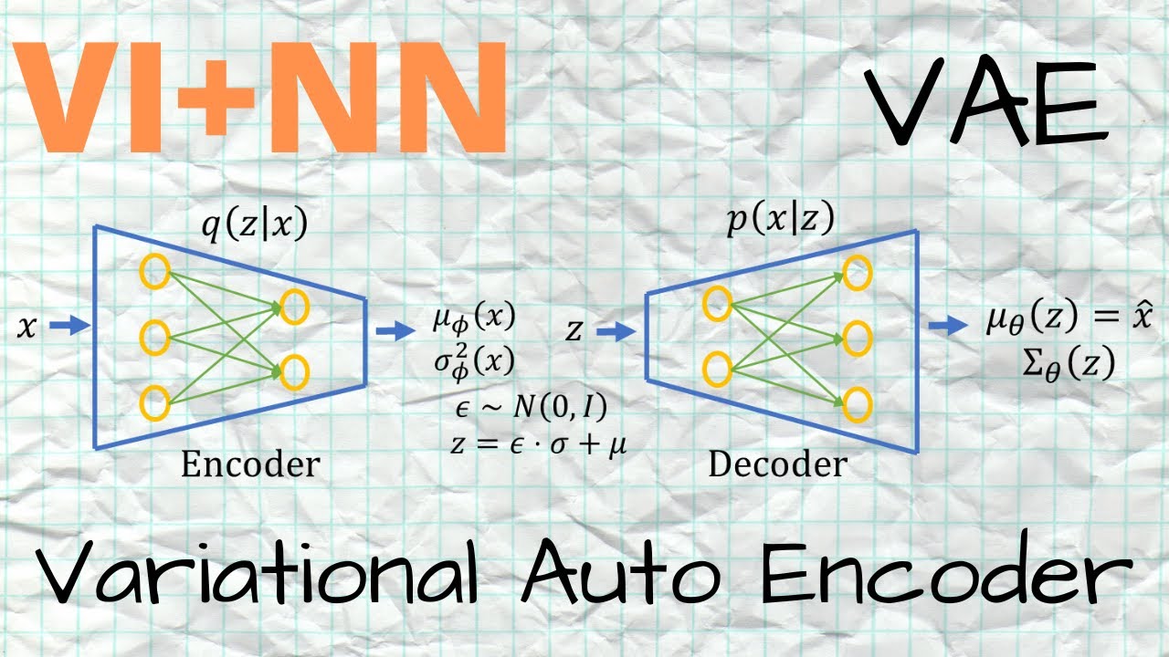
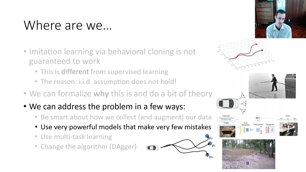
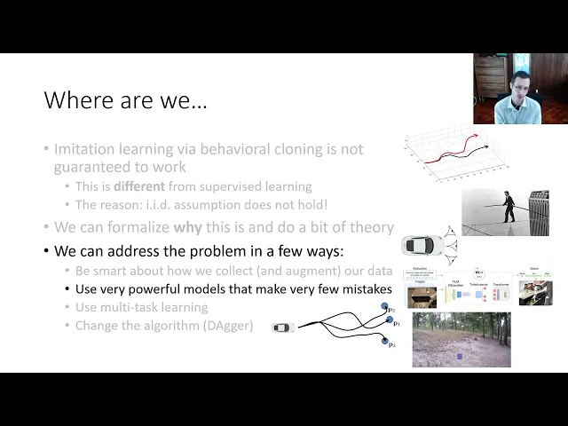
all right the remainder of today's lecture will focus on the more practical methods that can make behavioral cloning work as well as some other algorithms that we could use so we talked about a little bit of theory but now we'll talk about how the problem can be addressed in a few ways by being smart about collecting your data by using very powerful models that make comparatively fewer Mistakes by using multitask learning and by changing the algorithm and I'll go through these pretty fast so my aim with these uh with this portion of the lecture is not really to go in great detail about how to actually Implement some of these methods but just to give you a sense for the types of methodologies that people employ the one method that you will Implement in homework is dagger and I'll go through that somewhat more precisely okay so what makes behavioral cloning easy and what makes it hard as I mentioned in the previous part of the lecture if you have very perfect data then these accumulating errors are a big problem because as soon as you make even a small mistake you're outside of the distribution of perfect data but if you if you actually already have a bunch of mistakes in your data set and Corrections for those mistakes then when you make a small mistake you'll be in a state that is somewhat similar to other mistakes that you've seen in the data set and the labels in that portion of the data set will tell you how to correct that mistake so there are a few ways that you could leverage this Insight you could actually intentionally add mistakes and Corrections during data collection that's not actually an entirely crazy idea so the mistakes will hurt meaning that it will dilute the training set but the corrections will help and often the corrections help more than the mistakes hurt the reason for it is that if the mistakes are somewhat random they tend to average out meaning that the most optimal action is still the most probable however by making mistakes during data collection you force the expert to provide examples in more diverse States and that will teach the policy how to make Corrections the simplest version of this you can think of is if you force the expert to make a mistake with some probability independent of which state they're in then the mistakes will be largely uncorrelated with the state whereas the optimal action will be correlated with the state so when your neural network learns the action that correlates most of the state it will actually tend to learn the optimal action and avoid the mistakes but it will still benefit from seeing the corrections in those worse States another thing that we could do is use some form of data augmentation and that camera trip from before can be thought of as a kind of data augmentation essentially a method that adds some fake data that illustrates Corrections like those side facing cameras and that can be done with the by leveraging some sort of domain knowledge about the problem you're solving to create some additional fake data and roughly speaking the effect of these two tricks is kind of the same in both cases the aim is to provide examples in states that the expert is unlikely to visit but the policy might end up Landing in now there isn't really much more to this methodology than that so in discussing these tricks I'm going to just show you two examples of previous papers that use tricks like this to good effect so the first one I'll mention is a data augmentation based approach in this paper which focused on flying a drone through the forest so the output action space is discrete it's just go left go straight or turn right and here's a video from their work so they're going to fly these drones through hiking trails in Switzerland the this is a from the University of Zerg and the idea is pretty straightforward so they have a continent and they the kind that looks at the image and it predicts one of three discrete labels left right and straight now uh these are examples from the training set so they're labeled and where do they get the labels where well they get the labels uh by of course using lots of machine learning using lots of hiking trails but the data collection procedure is actually very straightforward they didn't actually have humans apply the quadcopter what they did instead is they got a person to walk the hiking trails and the person was let me fast forward here wearing a funny hat their hat had three cameras on it a forward-facing camera a left-facing camera and a right-facing camera and their approach was actually even simpler than the driving example they simply assumed that the person would always go in the correct direction and they labeled the left facing camera with the action to go right and the right facing camera with the action to go left and the straight facing camera with the action to go straight that's it that is the entirety of the method so there's no attempt to record the human's actions and that actually worked pretty well and I think this is a really nice illustration of how that data augmentation approach can enable imitation learning to work well and it wouldn't surprise me in the least if had they actually flown the quadcopter through the force and only use the forward-facing camera if their results would have actually been somewhat worse foreign so this is a similar thing with a handheld camera and here is their drone here's another interesting example this is a robotic manipulation example and here the authors of this paper are using a very low cost very cheap and relatively inaccurate arm and a very simplistic tele operation system based on a kind of a hand motion detector and they're teaching the robot various skills like using a cloth to wipe down a box of screwdrivers picking up and pushing objects things like this and they're using a game controller here and one of the things that they do is they illustrate a lot of mistakes in their demonstrations kind of inevitably just because they have such a low cost and imperfect to the operation system and because they illustrate so many mistakes they actually end up within a situation where the robot when it makes mistakes actually recovers from them so they have some examples where it picks up objects sometimes it picks them up incorrectly sometimes a human actually perturbs it but the robot is actually pretty good at recovering from perturbations including ones that are introduced by the person so here the person is missing but the robot just is unworried about that and keeps trying to do the task um so here it has to slide the wrench into a particular spot so sometimes imperfect data collection can actually be better than highly perfect data collection okay now that trick for getting behavioral cloning to work is um not very reliable and it takes a little bit of domain-specific expertise although it does provide a kind of a guidance anytime you're collecting data for imitation learning keep in mind that having ways to put the system in states where the expert can demonstrate Corrections can be a very good thing and it's also worth thinking about data augmentation trucks but let's talk about some more Technical Solutions why might you fail to fit the expert Behavior because if you can minimize the number that value Epsilon perhaps even Epsilon t squared might still be a small number so if you can understand why you might fail to fit the expert Behavior maybe you can get a model that's so powerful that it's probability of mistakes is so low that even that quadratic cost doesn't actually worry you too much so why might you fail to fit the expert well one reason is what I'll refer to as non-markovian Behavior non-markovian Behavior means that the expert doesn't necessarily choose the action based only on the current state second reason is multimodal behavior that means that the expert takes actions randomly and their distribution of reactions is very complex and might have multiple modes okay let's talk about the normal coping Behavior first so when we train a policy that is conditioned on the current observation but the policy is markovian in the sense that it assumes that the current observation is the only thing that matters it's basically assuming that the observation is the state that's not necessarily a problem if the expert also chose the action based only on the current observation but humans very rarely do that humans can't really make decisions entirely in the moment completely forgetting everything they saw before so if we see the same thing twice if we were perfectly markovianized agents we would do the same thing twice regardless of what happened before and that's pretty unnatural oftentimes humans will base their decision on all of the past things they saw for example if the human driver notices something in their blind spot and then looks back on the road they still remember what they saw in their blind spot or maybe even more problematic if someone just cut them off and they got a little flustered maybe they'll be driving a little differently for the next few seconds so generally humans are actually very non-markovic in the sense that humans human behavior is very strongly affected by the temporal context so if we're training a policy that only looks at the current image it's unaware of all that context and it might simply not be able to learn a single distribution that captures human behavior accurately because human behavior doesn't depend on just the current observation so how can we use the whole history well it's actually pretty straightforward we just need a policy representation that can read in the history of observations so we might have a variable number of frames and if we just simply combine all the frames into one giant image with like 3000 channels that might be difficult because you might have too many weights so what we would typically do is use some kind of sequence model so we would have our let's say if we're using images we would have our convolutional encoder if you're not using images you would have some other kind of encoder and you would encode all the past frames and then feed them through a sequence model such as an lstm or Transformer and then just predict the current action based on the entire sequence setting up these models is a little bit involved but there's actually nothing here that is special fermentation running so the same way that you might build a sequence model to process let's say videos in supervised learning exactly the same kinds of approaches can be used here whether it's lstms or Transformers or something else entirely like temporal convolutions again I won't talk about those architectural details in detail because they're actually not imitational money specific so anything that you learned about before for sequence modeling could just as well be used for imitation line there is however an important caveat that I want to mention which is that using histories of observations does not always make things better and the reason that it might sometimes make make things worse is that it might exacerbate correlations that occur in your data and this is a little bit of an aside I don't necessarily expect all of you to kind of to know this in detail but I do think it's an interesting aside and it's something that perhaps might Inspire some ideas for things like final projects why might this work poorly well here's a little scenario let's say that you have a a strange kind of car where there's a dashboard indicator for whether you're pressing the brakes so whenever you press the brakes there's a light bulb that lights up inside the cabin and the camera that is recording your data for imitation running is inside the cabin so the camera can see out of the window and it can also see the brake indicator so whenever the person steps on the brake the light lights up now in this case there's a person standing in front of the car and the driver stepped on the brakes because there was a person there but what the policy sees in the training data is it'll see one frame where the person is visible but the brake indicator is not uh is not on and the brake is pressed and then we'll see many steps after that where the brake indicator is pressed uh it is lit and the brake is pressed so there's a very strong association between the brake indicator and the brake being pressed if you have if you're reading in histories the situation is a lot worse because now you don't even need the brake indicator when you're reading in histories just the fact that the break was pressed in previous time steps is Apparent from looking at the sequential images you see the car slowing down you know the brake was pressed so the point is that the action itself correlates with future instantiations of that action if the information is somehow hidden then of course the policy is forced to pay attention to the important queue which is the fact that there's a person but if these auxiliary cues are present even though they are not the real cues that led to the action they serve to confuse the policy as a spurious correlation as a kind of causal confounder so the slowing down that you see when you look at history is caused by breaking but the policy might not realize that it might think that whenever you see the car slowing down that's indication that you should break in the same way as the brake indicator is the effect not the cause of braking but when you see lots of images of that correlation in there you might get confused so you can call this causal confusion it's discussed a little bit in this paper there are a few questions we could ask about this does including history mitigate causal confusion or does it make it worse uh and I'll I'll leave as an exercise for you at home another exercise is at the end of this lecture we'll talk about a method called dagger and after we talk about that I want you to come back to this uh point and think about whether the method dagger will actually address this problem or make it worse so I'll leave that as an exercise for you uh to think about all right so that's non-markovian Behavior you can address it by using histories keep in mind that that's not unequivocally always a good thing but if you're what you're worried about is non-markovian behavior that's the thing to do now let's talk about the other on multimodal Behavior that's kind of a subtle one let's say that you want to navigate around a tree and if you're flying a quadcopter you can fly around the tree to the left or you can fly around the tree to the right both are valid Solutions the trouble is that at that point when you're in front of the tree some expert trajectories might involve going left and some might involve going right so in general in your training data you'll see very different actions for very similar States now this is not a problem if you're doing something like that that Zurich paper where they use a discrete action space left right and straight because you can easily represent a distribution where there's high probability for left high probability for right and low probability for straight because you're directly outputting three numbers to indicate the probability of each of those actions however if you're outputting a continuous action maybe the mean and variance of a gaussian distribution now we have a problem because a gaussian has only one mode in fact if you see examples of left and examples of right and you average them together that's very very bad so how can we address this well we have a few choices we can use more expressive continuous distributions so instead of outputting the mean and variance of a single gaussian we can output something more elaborate or we can actually use discretization but make it feasible in high dimensional action spaces and I'll talk about both Solutions a little bit next so first let's talk about some examples of continuous distribution we can use and again I won't go into great detail about each of these methods so for details about how to actually Implement them I'll have some pointers and references and I would encourage you to look that up yourself if you want to actually try it my aim here is mostly to give you a survey level coverage of the different techniques so that you kind of know the right keywords and the right ideas okay so what we're going for is some way to set up a neural network so that it can output multiple modes for example a high probability of left high probability of right and low probability of going straight so we have a few options a very simple but maybe less powerful option is to use a mixture of gaussians and I'll talk about how to set that up with neural Nets I'm more sophisticated one is to use linked variable models and then something that has recently become very popular is to use diffusion models because the fusion models have gotten a lot more effective and a lot easier to train in recent years but let's start with a mixture of gaussians because that is probably the simplest thing to implement although it's not quite as powerful as the others so the idea here is the following a mixture of gaussians is uh can be described as a set of means covariances and weights okay so let's say you have n different uh gaussians that you want output let's say maybe it's n equals 10 let's say you're going to Output 10 means 10 covariances and a weight on each of those 10 mixture elements to indicate how large each of them is so you probably learn about mixed trip gaussians in the context of something like clustering where the means and the variances are just vectors and matrices that you learn here everything is conditional in the observation so your neural network is actually outputting the means and variances so they're not numbers that you store they're actually outputs of your neural net before our output was just the mean and maybe just one covariance Matrix now it's maybe going to be 10 vectors of means and 10 covariance matrices and a scalar weight on each of those 10 to indicate how large they are but in terms of implementing it it's actually pretty straightforward all we have to do is code up our neural network so it has all those outputs write down the equation for a mixture of gaussians take its logarithm as our uh training objective and optimize it the same way that we did before so uh the way that you would implement this in let's say Pi torch is you would literally implement the equation for a mixture of gaussians take its log and use that as your training objective just don't forget to put a minus sign in front if you're minimizing it so that's basically the idea your neural net outputs means covariances and weights and Modern Auto devtools like pytorch actually make this pretty easy to implement of course the problem with a mixture of gaussians is that you choose a number of mixture elements and that's how many modes you have so if you have 10 mixture elements and you want 10 modes that's fine but what if you have 100 modes what if you have extremely high dimensional action spaces perhaps you're not driving a car but you're controlling a humanoid robot with the Degreaser freedom and you want a thousand different modes now you have to do something a little smarter latent variable models provide us a way to represent a much broader class of distributions in fact you can actually show that latent variable models can represent any distribution as long as the neural network is big enough the idea behind a latent variable model is that the output of the neural net is still a gaussian but in addition to the image it receives another input which is sampled from some prior distribution like a zero mean unit variance gaussian so you can think of it as almost like a random C the random seed is passed into the network and for different random seeds it'll output different modes so for example if we out if if we have a three-dimensional uh random Vector that we put in if we put in this random Vector we get this mode if we put in this random Vector then we get this other mode we'll train the network so that for different random vectors it outputs different modes now unfortunately you can simply naively take the network and feed in random numbers and expect it to do this because if you give it random numbers those random numbers aren't actually correlated with anything in the input or output so if you just do this in the most obvious way the neural net will actually ignore those numbers so the trick in training latent variable models is to make those numbers useful during training the most widely used type of method for this is what's called a conditional variational autoencoder we'll discuss conditional variational Auto encoders in great detail much later on in the course in the second half so I won't actually describe how to make this work right now but the high level intuition is during training the values of those random vectors that go into the network are not actually chosen randomly instead they're chosen in a smart way to correlate with which mode you're supposed to Output so the idea is that during training you figure out this particular training example has the left mode this training example has the right mode and you assign them different random vectors so the neural net learns that can pay attention to those random vectors because they tell it which mode to Output that's the intuition the particular technical way of making this work is a little bit more involved and requires more technical background so we'll talk about that in the second half of the course but the high level idea behind variable models is that you have an additional input of the model and that additional input tells it which mode to Output and then of course a test time if you want to actually make this work you can choose that random variable at random and then you'll randomly choose to go around the treat on the left or on the right Okay the third class of distributions I'll talk about which has gotten a lot of attention in recent years because these kinds of models have started working really well is diffusion models the fusion models are somehow similar to latent variable models but there's some differences so some of you might have heard about diffusion models as a way of generating images so things like Dali stable diffusion those are all methods that use diffusion models for image generation the way that diffusion models work for image generation and this is a very high level summary so if you're this feels vague to you it's because it is I Could Teach an entire class into future models in principle but for the purpose of covering it in two slides I'm going to provide a very high level overview let's say that we have a particular training image I'm going to denote the training image as x0 and the subscript here doesn't know time it actually denotes Corruptions of the image so x0 is the least corrupted XT is the most corrupted so x0 is the true image in a diffusion model you construct a fake training set where you add noise to the image and then you train the model to remove that noise so the image x i plus 1 is going to be the image x i plus noise so X1 is x0 which is a True Image plus noise X2 is X1 which has some noise added and it adds even more noise to it and if you take an image and you add these different amounts of noise now you have a training set where you can teach a neural network to go backwards so the learn Network looks at the image x i and it predicts x i minus 1. so it's going to look at the slightly noisy image X1 and predicts x0 it's going to look at the slightly more noisy image X2 is going to predict X1 and so on and so on in reality we actually often train it to go all the way back to x0 so there's a choice to be made there but for Simplicity it helps to think about it as just going back one step and in reality what we actually predict is just the noise itself and that's not actually that different because if you predict x i minus 1 well you can get that by just predicting the noise and just subtracting the noise from X I so you can either have f of x I direct output x i minus one or you can have M of x i output the noise in which case x i minus one is just x i minus f of x i and that's a much more common choice to make okay now this is image garbage what we actually want to do is not generate images we want to of course generate actions so what we can do is we can extend this framework to handle actions Now actions of course also have a temporal subscript so I'm going to use the subscript T to denote time in the temporal process for control and I'm going to use the second subscript to denote the diffusion time step so a t comma 0 is the true action in the same way that x0 was the True Image a t comma I plus 1 is ATI plus noise and just like before we can learn a network that now takes in the current observation or state St and ATI and it outputs ATI minus 1. or just like before we would actually get a top of the noise so then ATI minus 1 is ATI minus F of s t ATI so the training setup is produced by taking all the actions adding noise to them teaching the network to predict what that noise was while also looking at the image and then a test time if we want to actually figure out the action then we feed in completely random noise and run this model for many steps to get it to denoise so turning the network over on the side it gets its input ATI it outputs ATI minus one which is a slightly denoised version of that action and it also gets to look at the image we start off with noise at test time we feed that into this box as the for as the first value of ATI and then we repeat this process we denoise it put it back in denoise some more and repeat this process many times and then at the end out comes a clean glue to action and during training we add all this noise to ground shoot actions and we teach the network to undo the noise so that's the essential idea of a diffusion model actually implementing it takes a number of additional design decisions which I won't have time to go into here but I'll reference some papers and you can look at those papers for details the last trick I'm going to talk about is discretization discretization is in general a very good way to get complex distributions but it's very difficult to apply discrimination naively in high Dimensions so remember in that Zurich paper where the actions were to go left go right and go straight this multimodality problem basically didn't exist but of course that was for 1D actions in higher Dimensions if you have let's say 10 dimensional actions discretizing the action spaces impractical because the number of bins you need increases exponentially with the number of dimensions so the solution is to discretize one dimension at a time and that's the idea behind Auto regressive discretization so here's how we can do it let's say our action is a three-dimensional vector I'm going to use at 0 to node Dimension 0 81 to no Dimension 1 and 82 to denote the dimension 2.
don't be confused with the notation from diffusion models before this has nothing to do with that so the second number is just the dimension and it's just a scalar value right so here's how we're going to set up our Network we take the image and we encode it with some kind of encoder like content and then we'll put into a sequence model which could be a Transformer or an lstm so whatever your favorite sequence model is and at the first step of the sequence we output Dimension zero and we can discretize Dimension zero uh just into bins right so it's just one dimension discretizing a number line is pretty easy so we have one bin for every possible value you could have ten bins you could have 100 bins since it's one dimensional that's very easy to do and then at the second time step in the sequence we feed in the value at 0 and we output at1 again with a discretization and then the next time step we output we input 81 and we output 82. so just like in a sequence model and something like a language model you would uh output the next token the next letter here you would output the next dimension of the action space and now each Dimension is discretized and the number of bins is no longer exponential in the dimensionality it's actually still linear in the dimensionality and then a test time if we want to sample then we do exactly what we do with any other sequence model is instead of feeding in the ground truth value of each Dimension which we don't have we would feed in the prediction from the previous time step again this is exactly the same as any other sequence model like language models for example so one way to implement is actually with a GPT style decoder only model now why does this work well the reason that this is a perfectly valid way to represent complex distributions is that it can be seen by looking at what probabilities actually predict at each step so the first time step predicts P of at 0 given St because you get an you get STS input and your output is at 0. the Second Step predicts the probability of at1 given stn and at 0.
so the dependence on St comes from the fact that it's passed in through the sequence model and at 0 is fed as input the third time step you predict 82 given st0 and 81.
![[AUTOML23] A Tutorial on MetaReinforcement Learning](https://img.youtube.com/vi/XUQ9jLOZqGc/maxresdefault.jpg)